Advanced Statistical Inference
EURECOM
\[ \require{physics} \definecolor{input}{rgb}{0.42, 0.55, 0.74} \definecolor{params}{rgb}{0.51,0.70,0.40} \definecolor{output}{rgb}{0.843, 0.608, 0} \definecolor{vparams}{rgb}{0.58, 0, 0.83} \definecolor{noise}{rgb}{0.0, 0.48, 0.65} \definecolor{latent}{rgb}{0.8, 0.0, 0.8} \]
\[ \require{physics} \definecolor{input}{rgb}{0.42, 0.55, 0.74} \definecolor{params}{rgb}{0.51,0.70,0.40} \definecolor{output}{rgb}{0.843, 0.608, 0} \definecolor{vparams}{rgb}{0.58, 0, 0.83} \definecolor{noise}{rgb}{0.0, 0.48, 0.65} \definecolor{latent}{rgb}{0.8, 0.0, 0.8} \]Setup: I toss the coin \(n\) times and observe \(\textcolor{output}{y}\) heads
Question: is the coin fair? What is the probability of heads?
Steps:
Assumptions: (1) the probability of heads is the same for all tosses and (2) each coin toss is independent of the others.
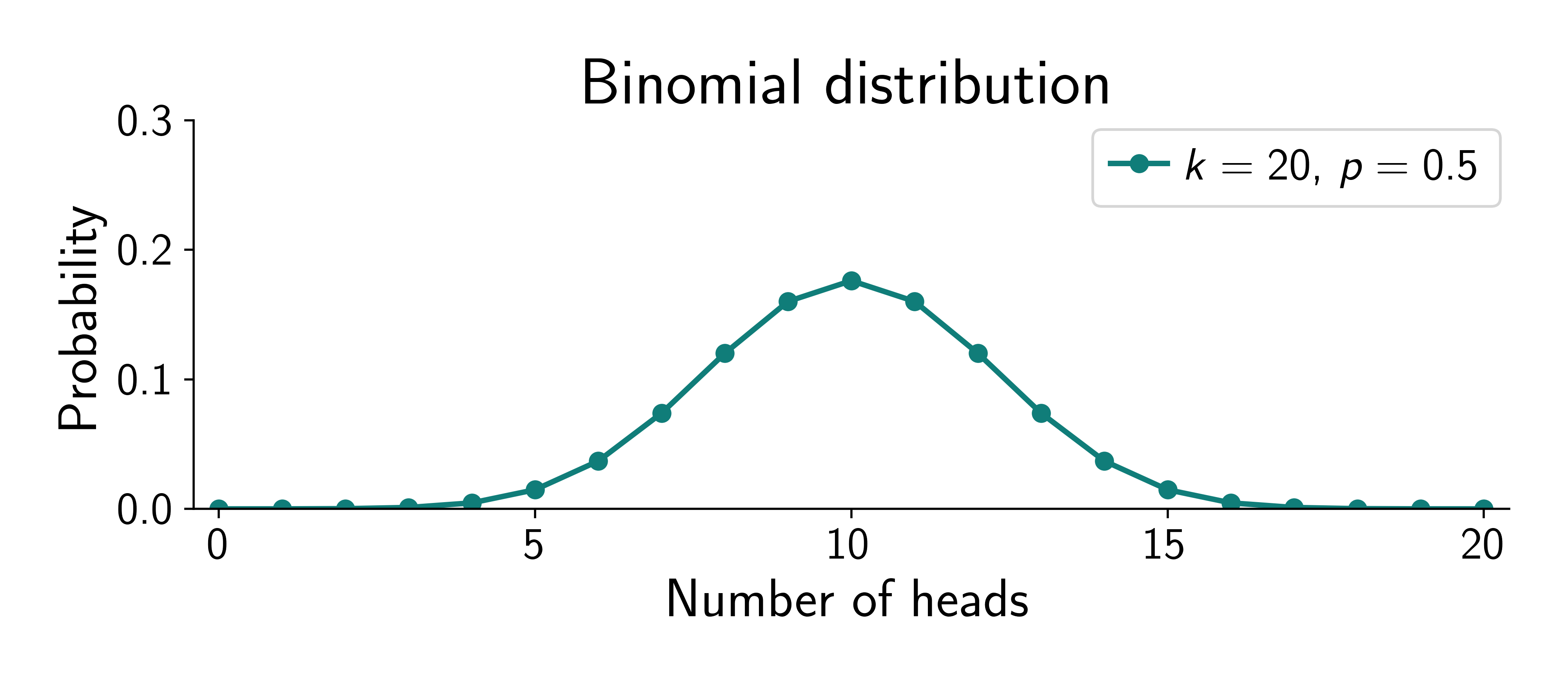
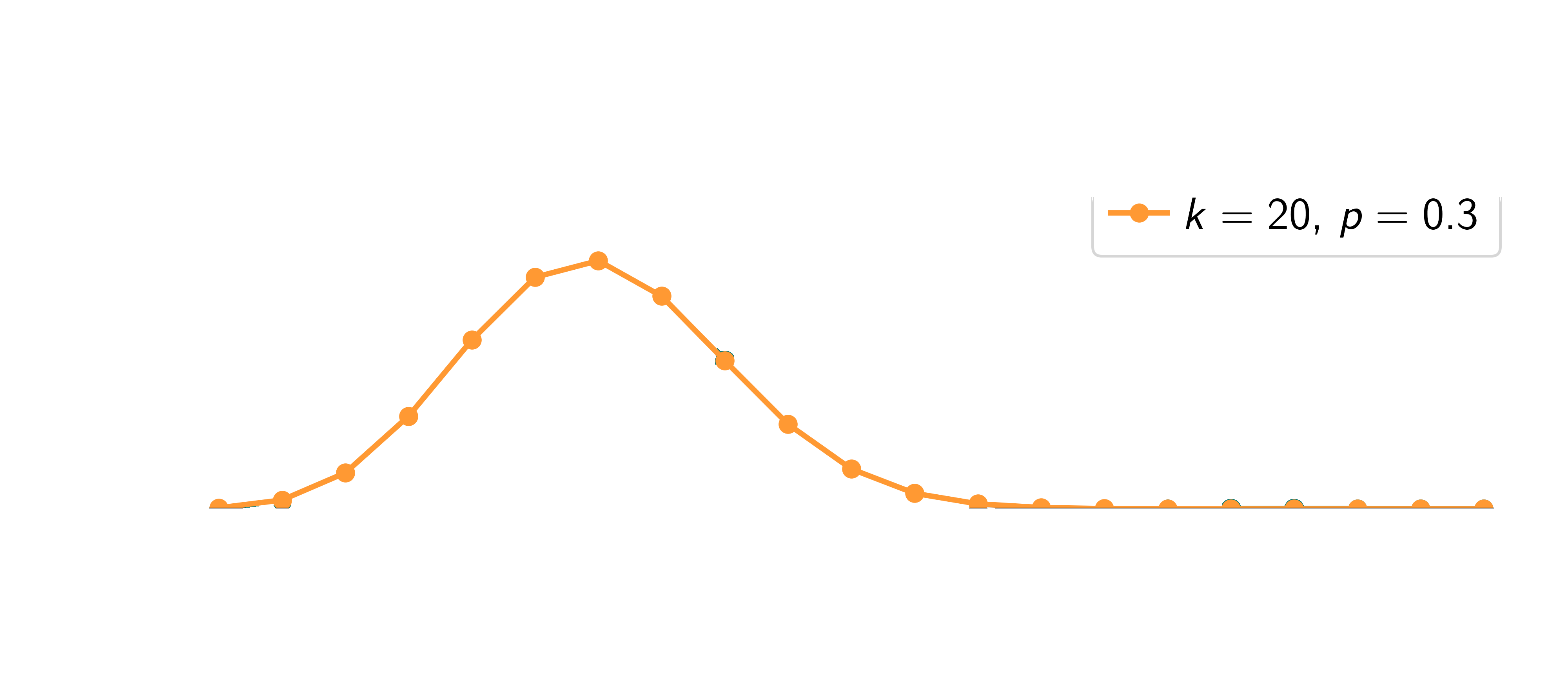
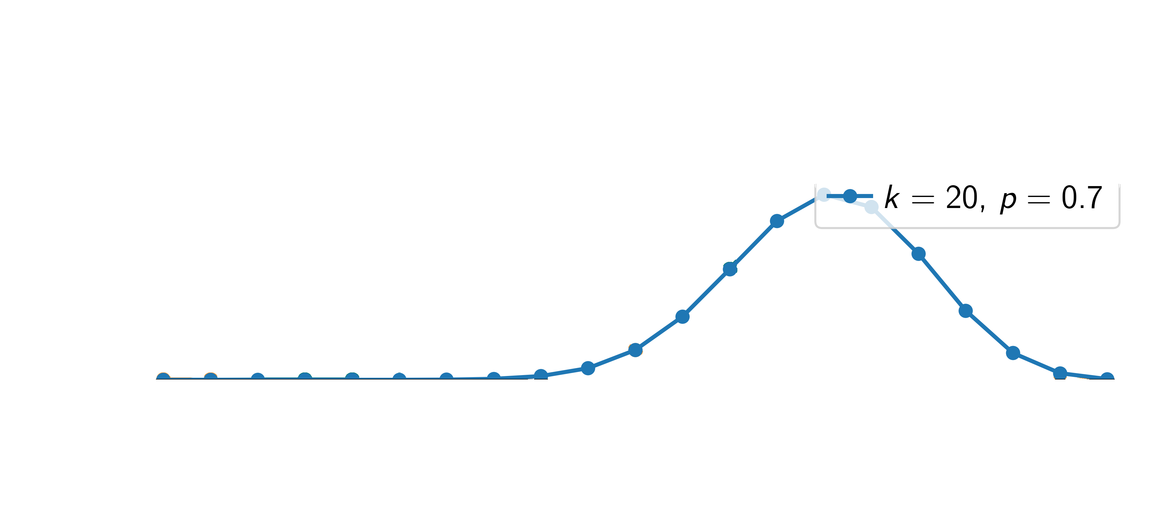
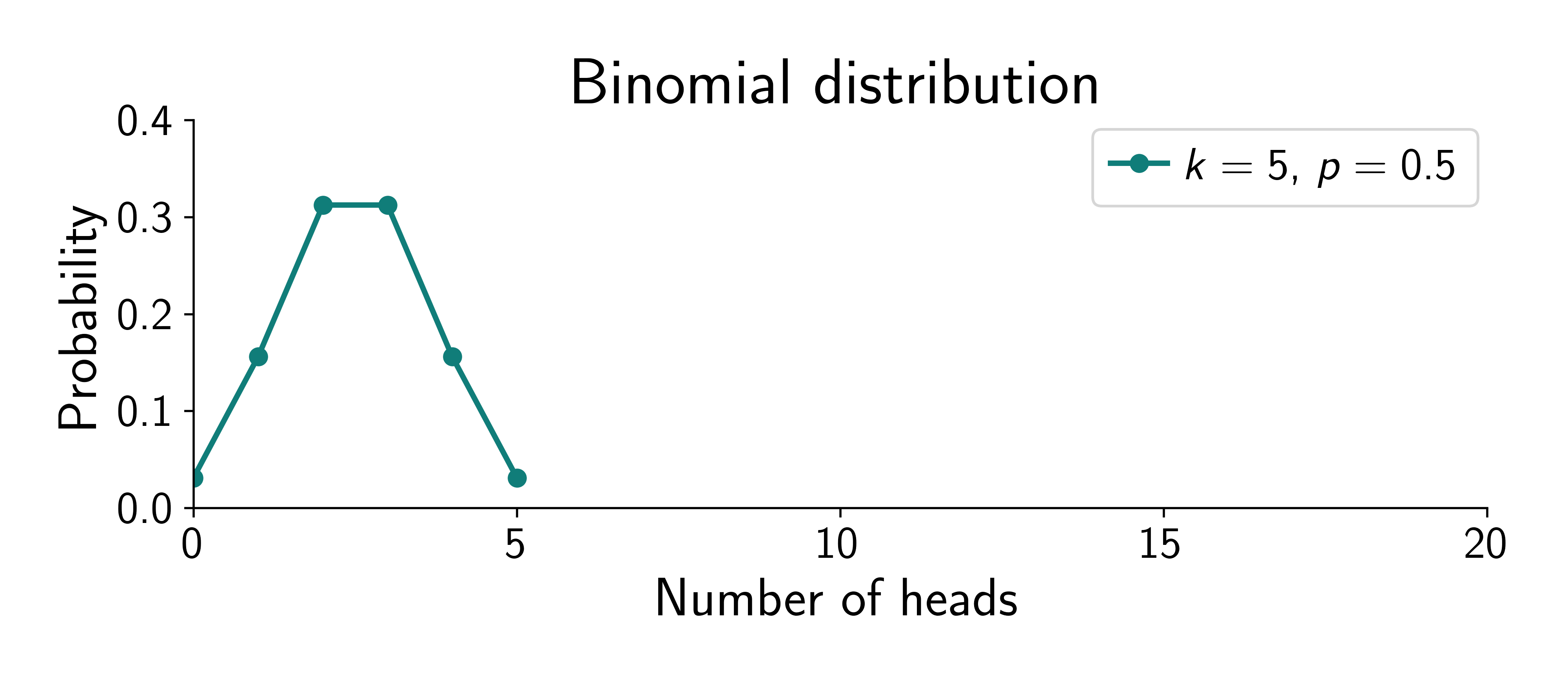
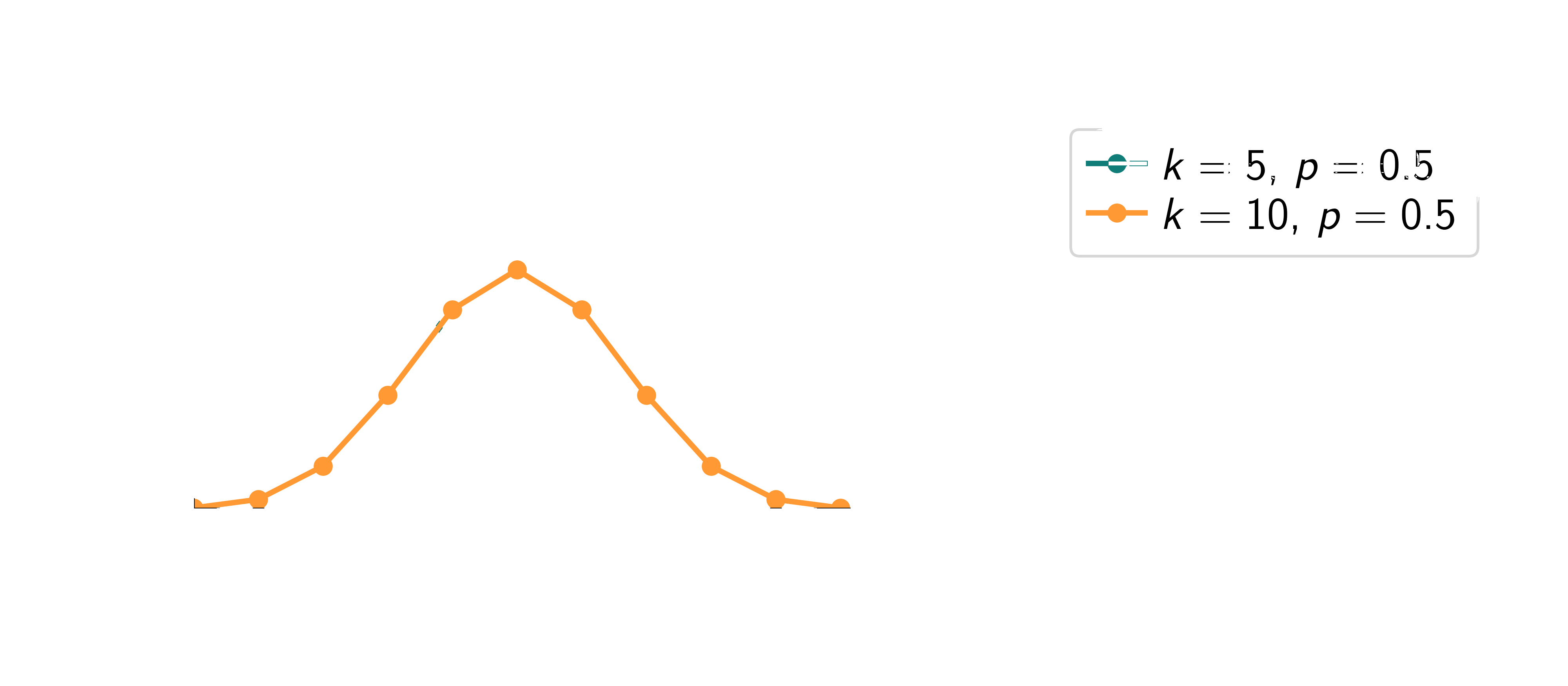
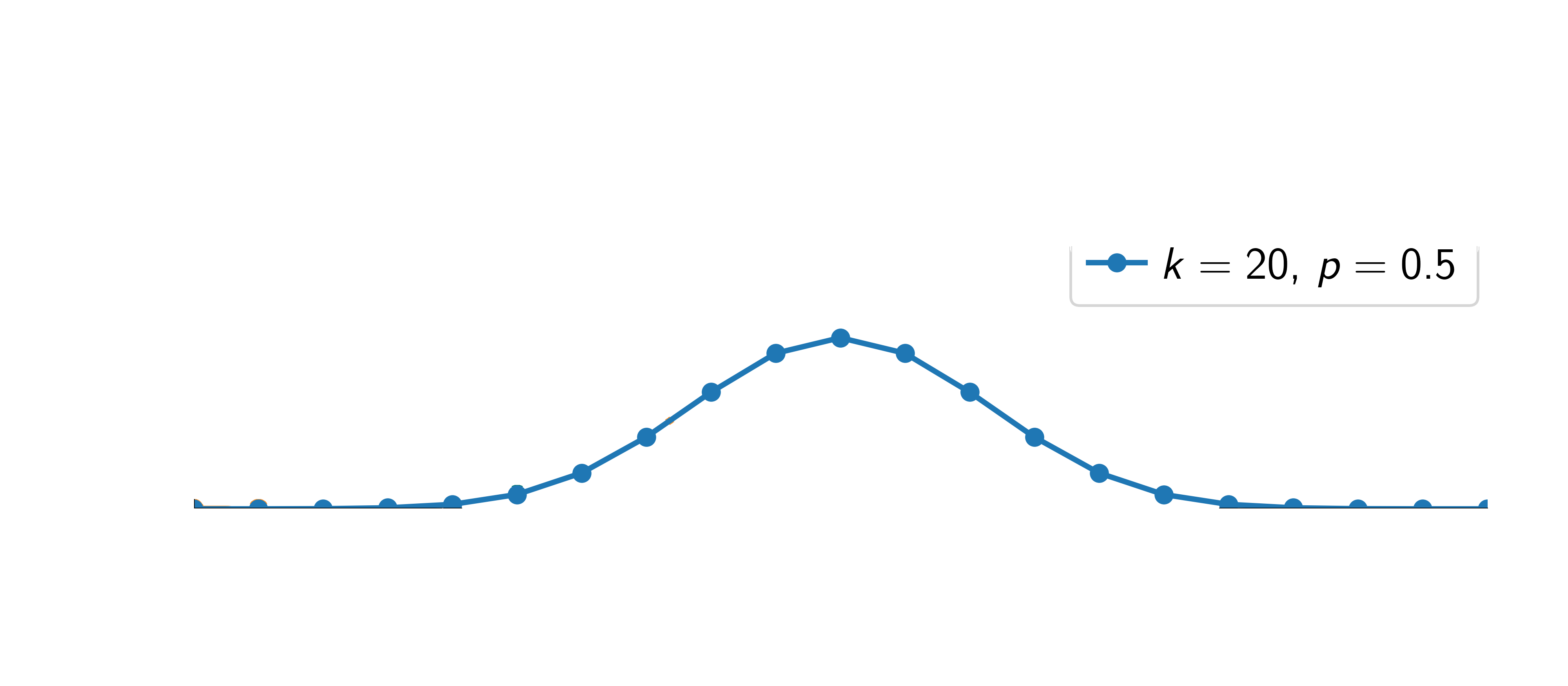
We can model the number of heads \(\textcolor{output}{y}_n\) as a binomial distribution with probability \(\textcolor{params}{\theta}\):
\[ p(\textcolor{output}{y}\mid \textcolor{params}{\theta}) = \binom {n}{\textcolor{output}{y}} \textcolor{params}{\theta}^{\textcolor{output}{y}} (1-\textcolor{params}{\theta})^{n-\textcolor{output}{y}} \]
where \(\textcolor{params}{\theta}\) is the probability of heads, \(n\) is the number of tosses, \(\textcolor{output}{y}\) is the number of heads and \(\binom {n}{\textcolor{output}{y}}= \frac{n!}{\textcolor{output}{y}!(n-\textcolor{output}{y})!}\) is the binomial coefficient.
We need to specify a prior distribution for \(\textcolor{params}{\theta}\).
How to choose it? Remember what \(\textcolor{params}{\theta}\) represents: the probability of heads.
It must be between 0 and 1.
It must represent a continuous distribution.
We want to be able to compute the posterior distribution (conjugate prior to the binomial distribution).
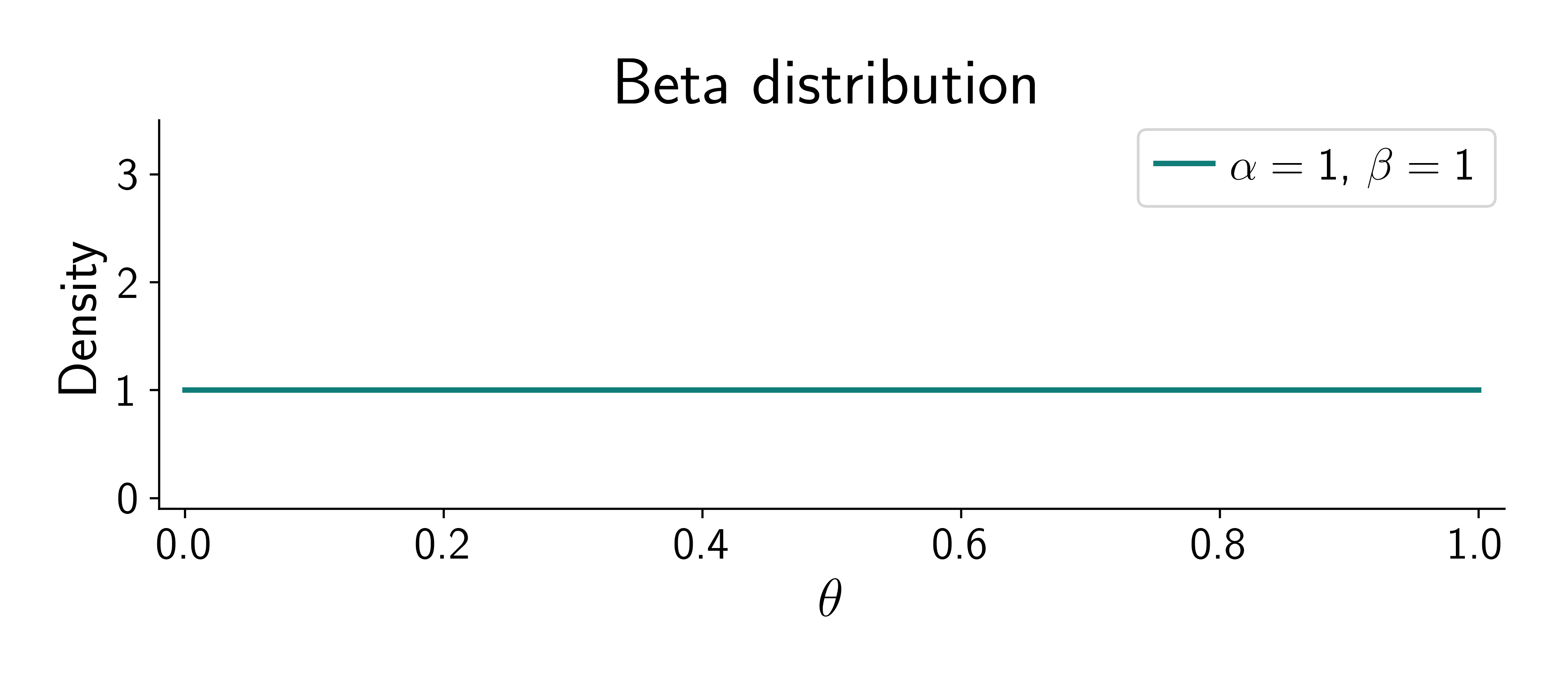
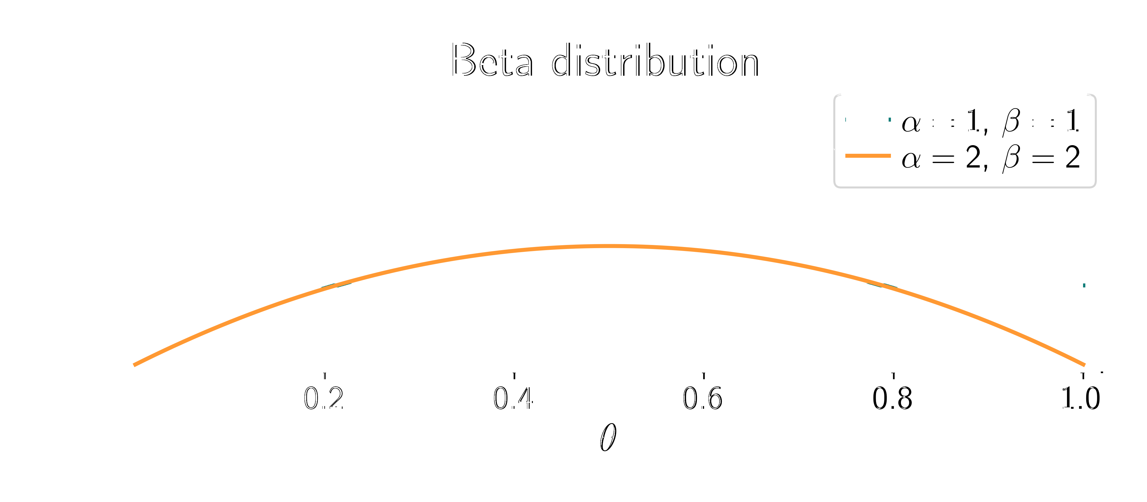
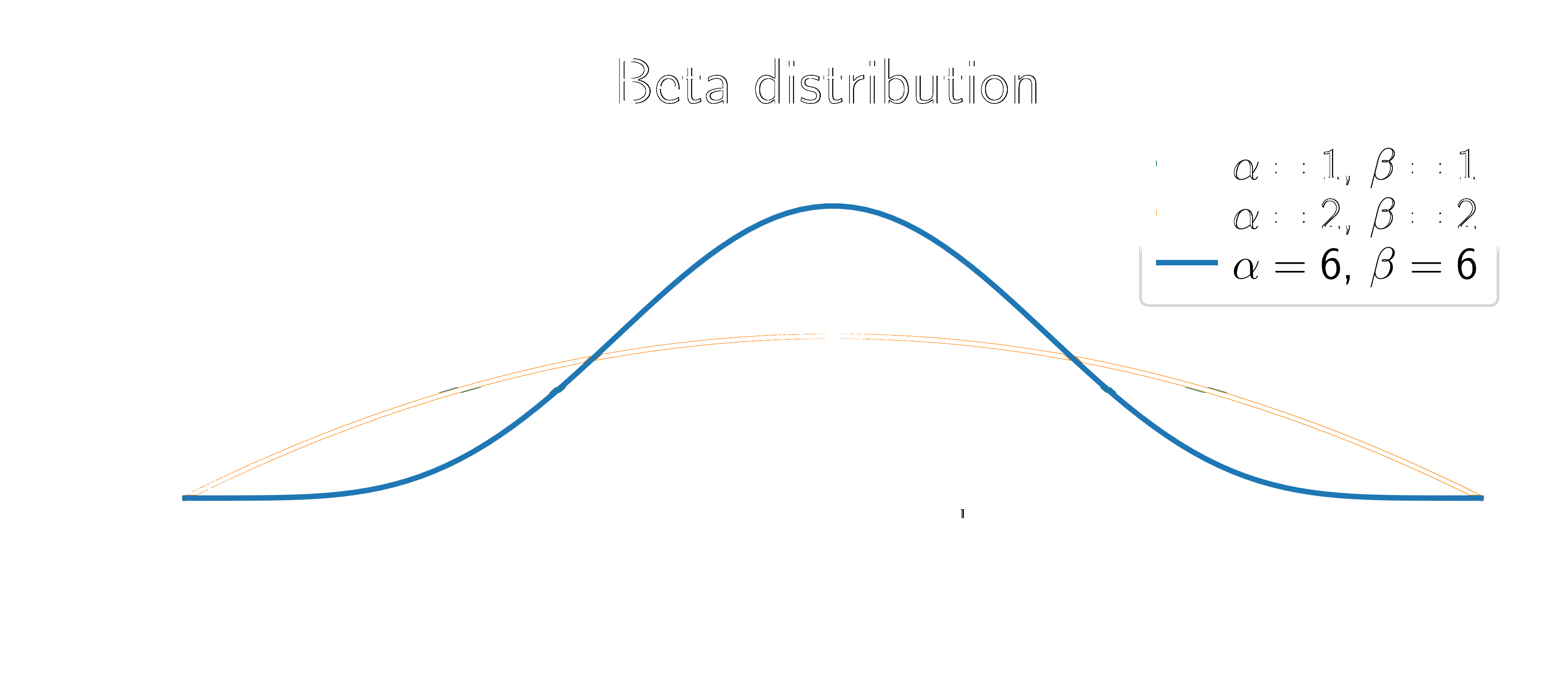
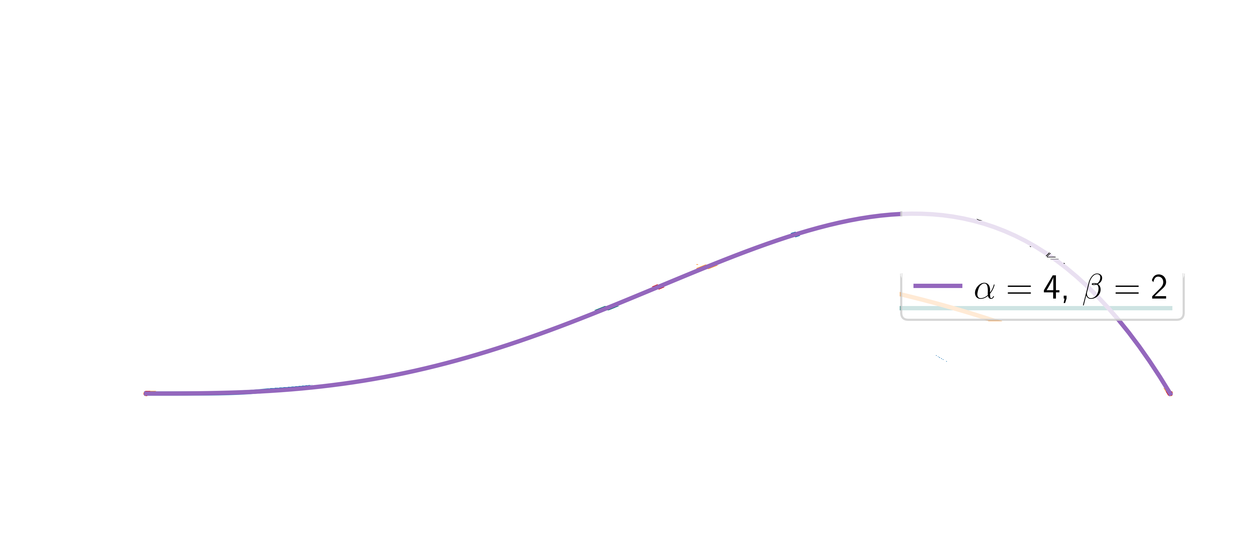
Beta distribution:
\[ p(\textcolor{params}{\theta}) = \frac{1}{B(\alpha, \beta)} \textcolor{params}{\theta}^{\alpha-1} (1-\textcolor{params}{\theta})^{\beta-1} \]
where \(B(\alpha, \beta) = \frac{\Gamma(\alpha)\Gamma(\beta)}{\Gamma(\alpha+\beta)}\) is the beta function and \(\Gamma(\cdot)\) is the gamma function.
Two parameters: \(\alpha\) and \(\beta\). They represent our prior beliefs about the probability of heads.

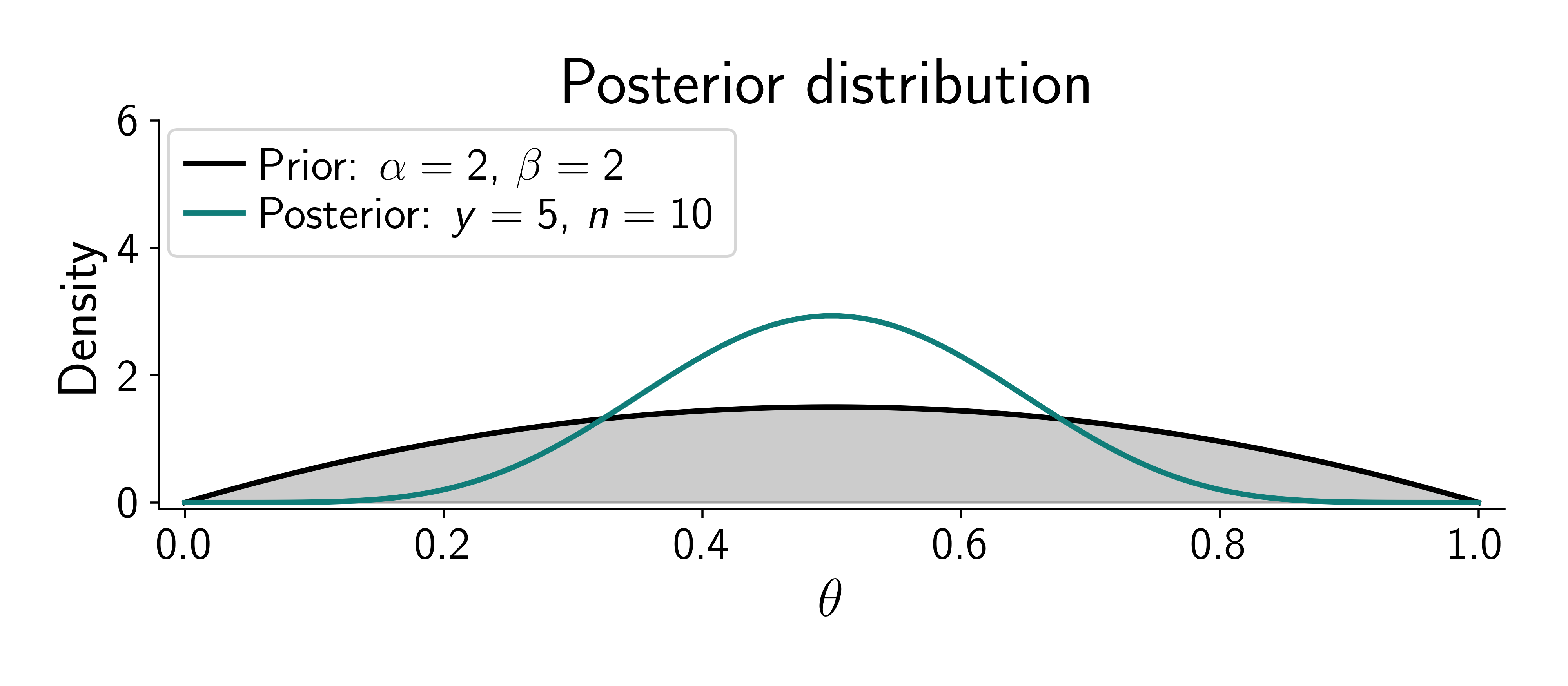
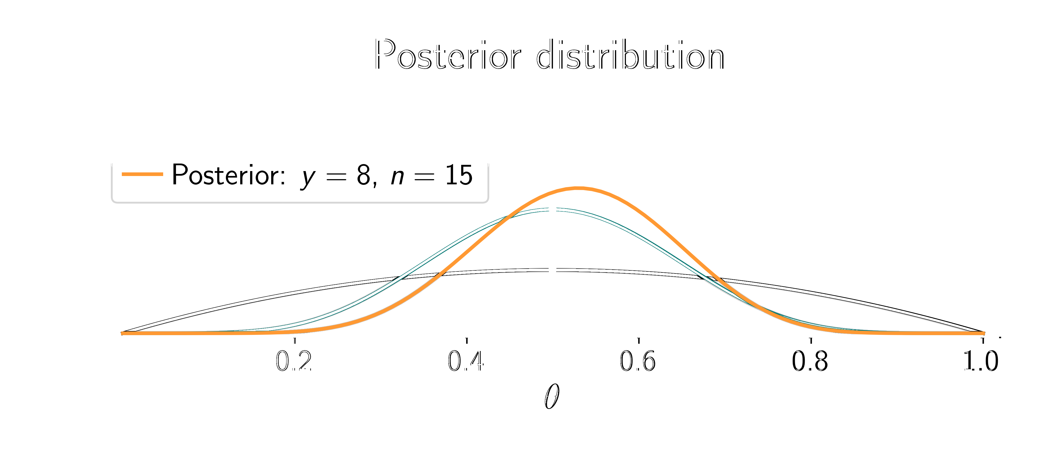
The posterior distribution is given by Bayes’ theorem:
\[ p(\textcolor{params}{\theta} \mid {\textcolor{output}{\boldsymbol{y}}}) = \frac{p({\textcolor{output}{\boldsymbol{y}}}\mid \textcolor{params}{\theta}) p(\textcolor{params}{\theta})}{p({\textcolor{output}{\boldsymbol{y}}})} \]
where \(p(\textcolor{output}{y})\) is the marginal likelihood (normalization constant).
Because the beta distribution is the conjugate prior to the binomial distribution, the posterior is also a beta distribution:
\[ p(\textcolor{params}{\theta} \mid \textcolor{output}{y}) = \frac{1}{B(\alpha', \beta')} \textcolor{params}{\theta}^{\alpha'-1} (1-\textcolor{params}{\theta})^{\beta'-1} \]
We need to compute the new parameters \(\alpha'\) and \(\beta'\).
From the conjugacy property, we have:
\[ p(\textcolor{params}{\theta} \mid \textcolor{output}{y}) = \frac{1}{B(\alpha', \beta')} \textcolor{params}{\theta}^{\alpha'-1} (1-\textcolor{params}{\theta})^{\beta'-1} \]
From Bayes’ theorem:
\[ p(\textcolor{params}{\theta} \mid \textcolor{output}{y}) \propto \textcolor{params}{\theta}^{\textcolor{output}{y}} (1-\textcolor{params}{\theta})^{n-\textcolor{output}{y}} \textcolor{params}{\theta}^{\alpha-1} (1-\textcolor{params}{\theta})^{\beta-1} \]
We can identify the parameters of the posterior distribution:
\[ \alpha' = \alpha + \textcolor{output}{y}, \quad \beta' = \beta + n - \textcolor{output}{y} \]
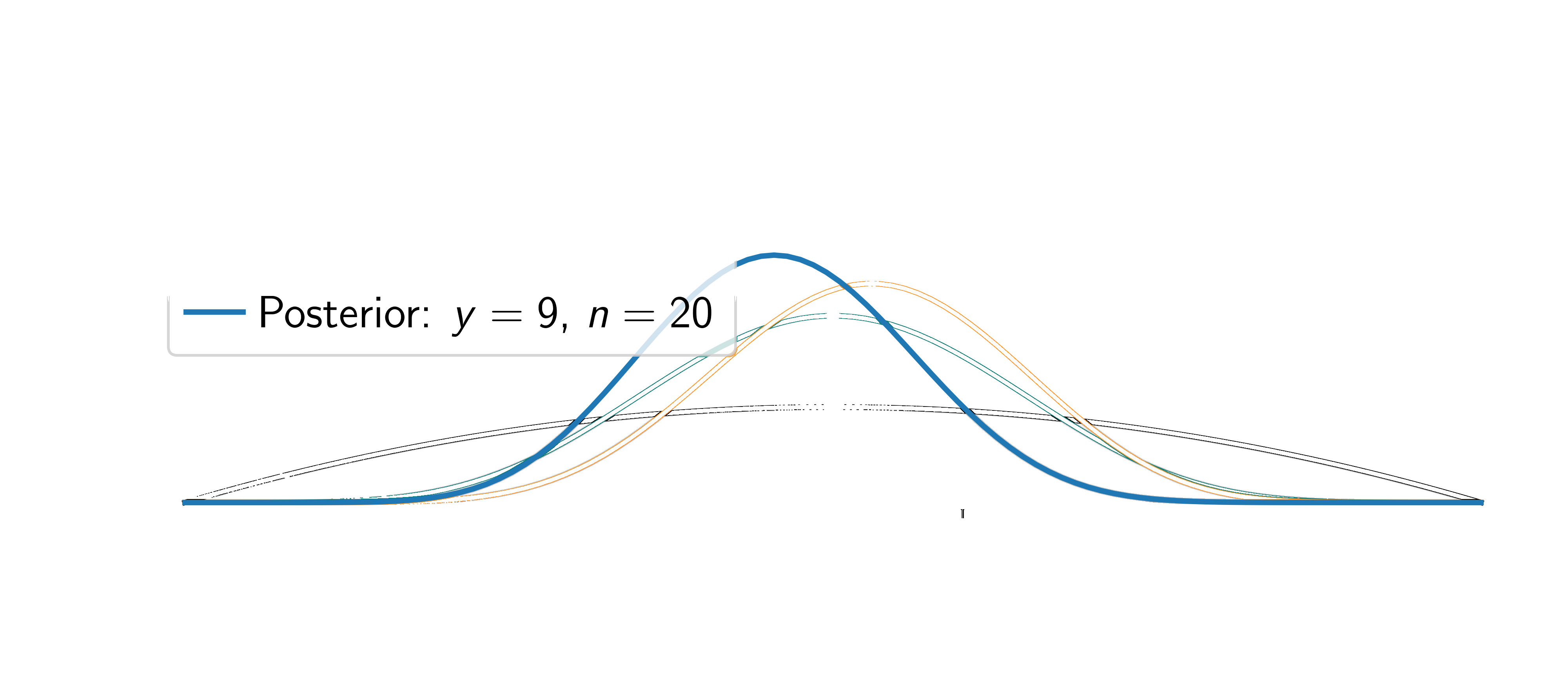
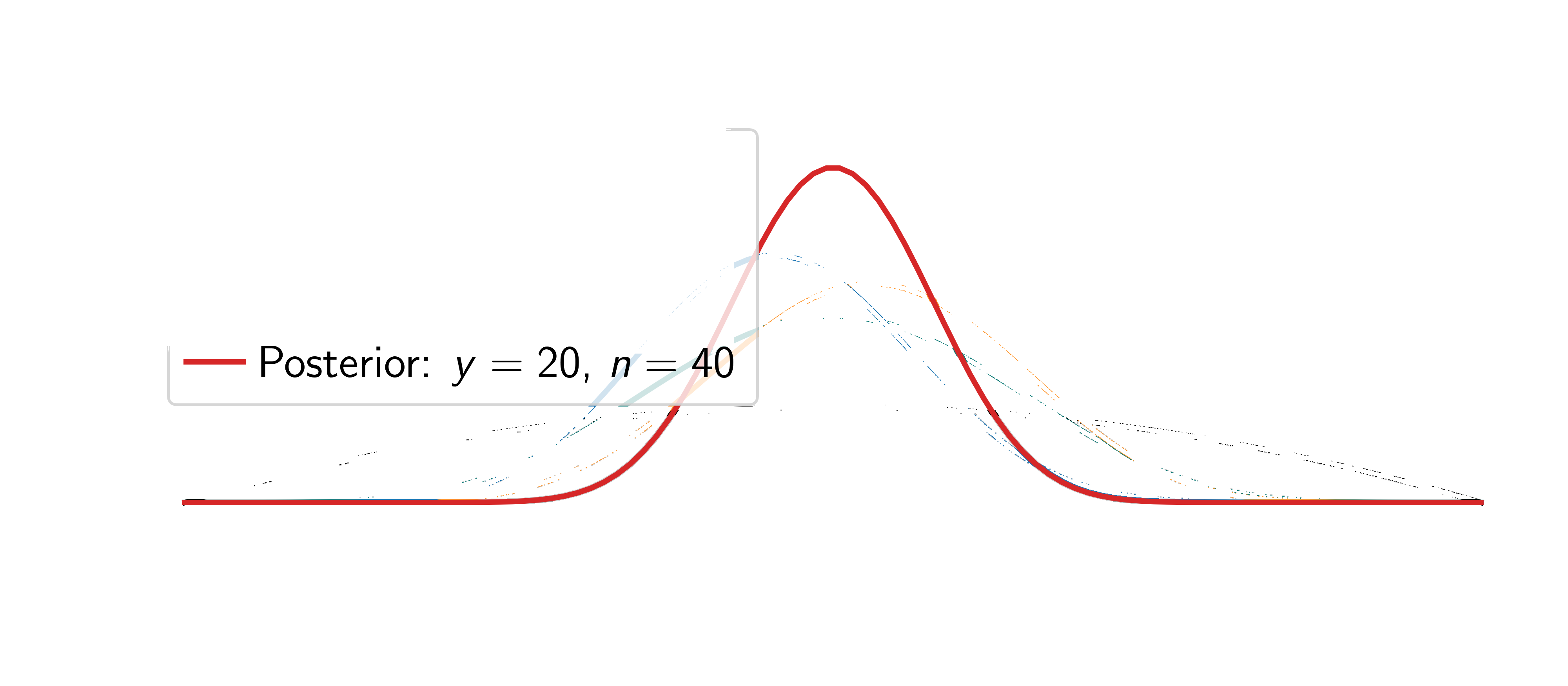
Assume the coin is fair (\(\textcolor{params}{\widehat\theta} = 0.5\)).
Two things happen:
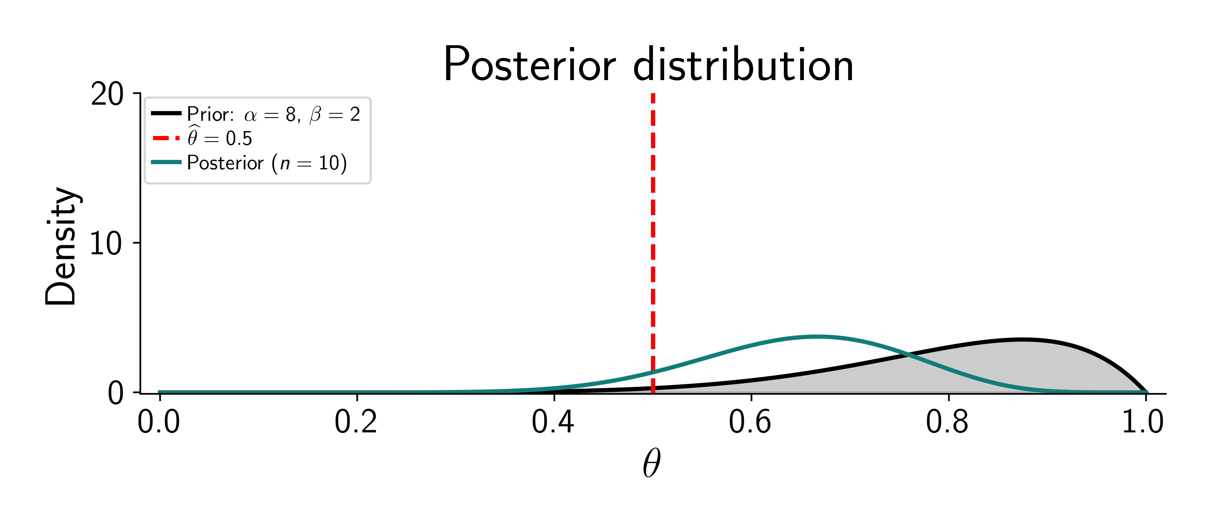
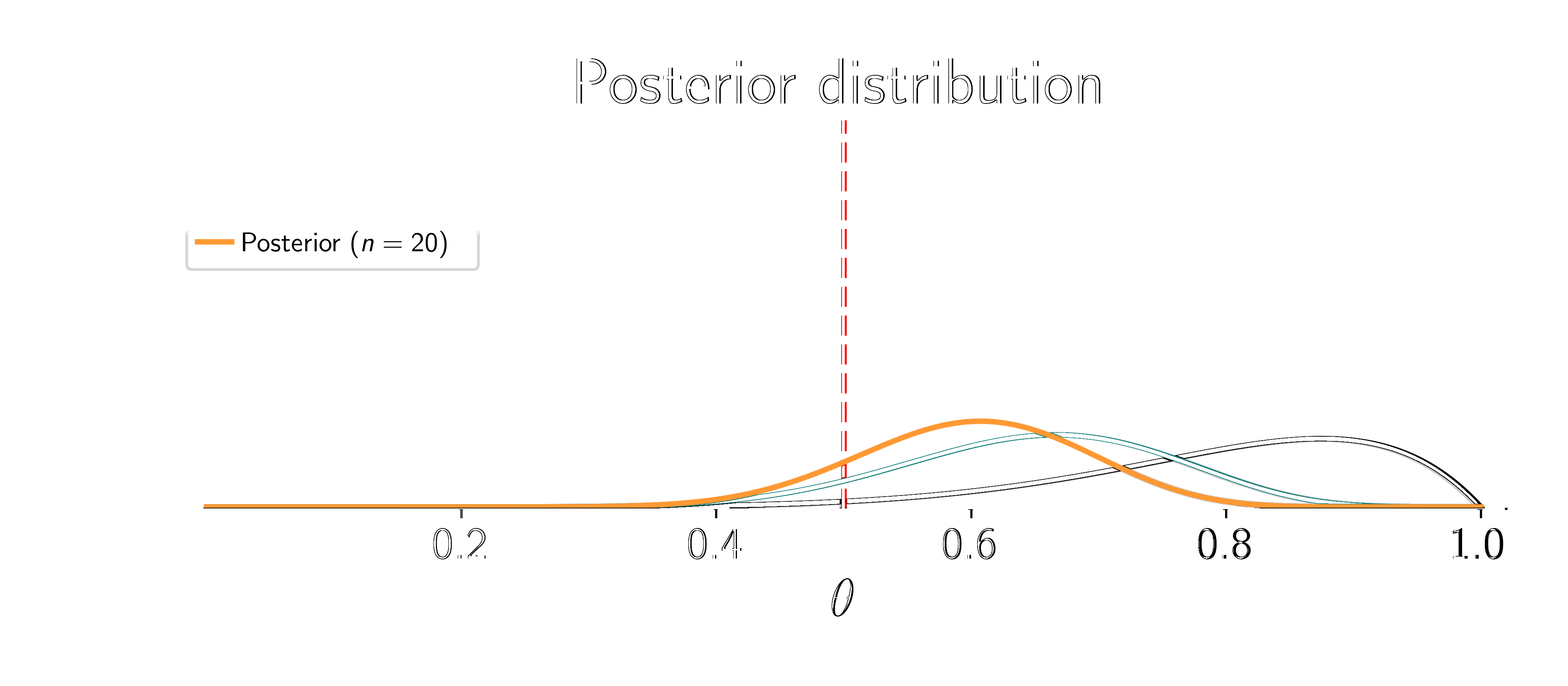
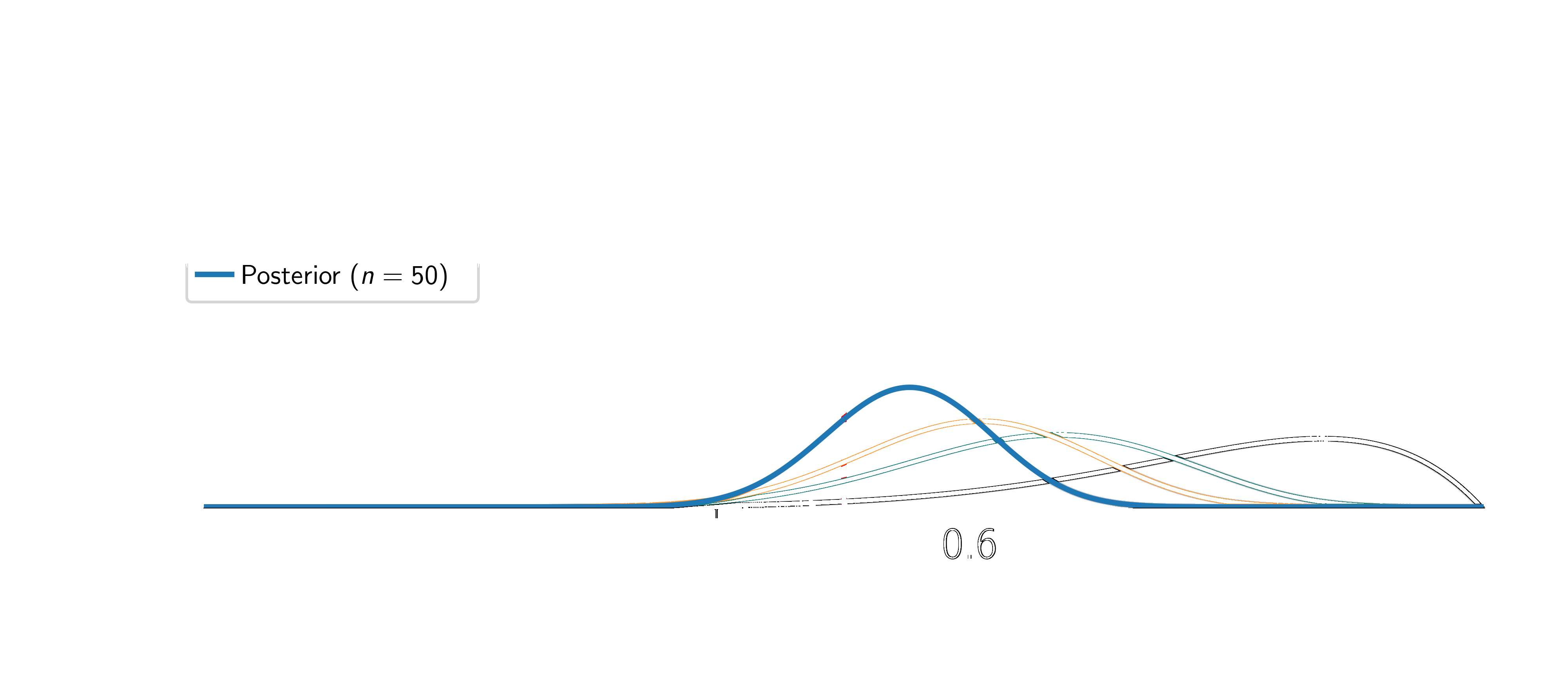
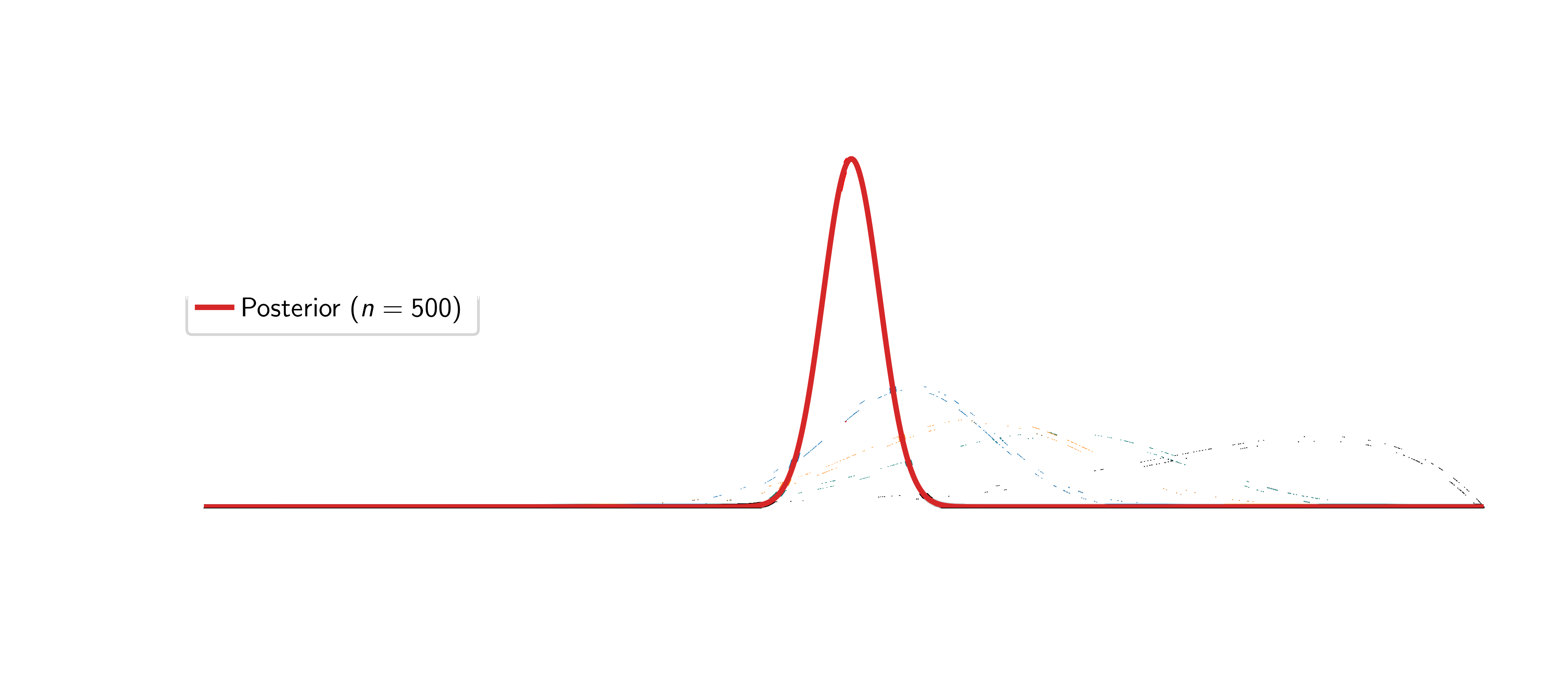
![]()
Simone Rossi - Advanced Statistical Inference - EURECOM