


Advanced Statistical Inference
EURECOM
\[ \require{physics} \definecolor{input}{rgb}{0.42, 0.55, 0.74} \definecolor{params}{rgb}{0.51,0.70,0.40} \definecolor{output}{rgb}{0.843, 0.608, 0} \definecolor{vparams}{rgb}{0.58, 0, 0.83} \definecolor{noise}{rgb}{0.0, 0.48, 0.65} \definecolor{latent}{rgb}{0.8, 0.0, 0.8} \]
\[ \require{physics} \definecolor{input}{rgb}{0.42, 0.55, 0.74} \definecolor{params}{rgb}{0.51,0.70,0.40} \definecolor{output}{rgb}{0.843, 0.608, 0} \definecolor{vparams}{rgb}{0.58, 0, 0.83} \definecolor{noise}{rgb}{0.0, 0.48, 0.65} \definecolor{latent}{rgb}{0.8, 0.0, 0.8} \]We have seen:
Gaussian processes (GPs) are a flexible and powerful tool for regression (and classification).
Linear models require us to specify a set of basis functions and their coefficients.
Can we use Bayesian inference to let the data decide?
Gaussian processes work implicitly with an infinite-dimensional set of basis functions and learn a probabilistic combination of them.
Gaussian processes can be explained in two ways:
Weight-space view: as a Bayesian linear regression model with a potentially infinite number of basis functions.
Function-space view: as a distribution over functions.
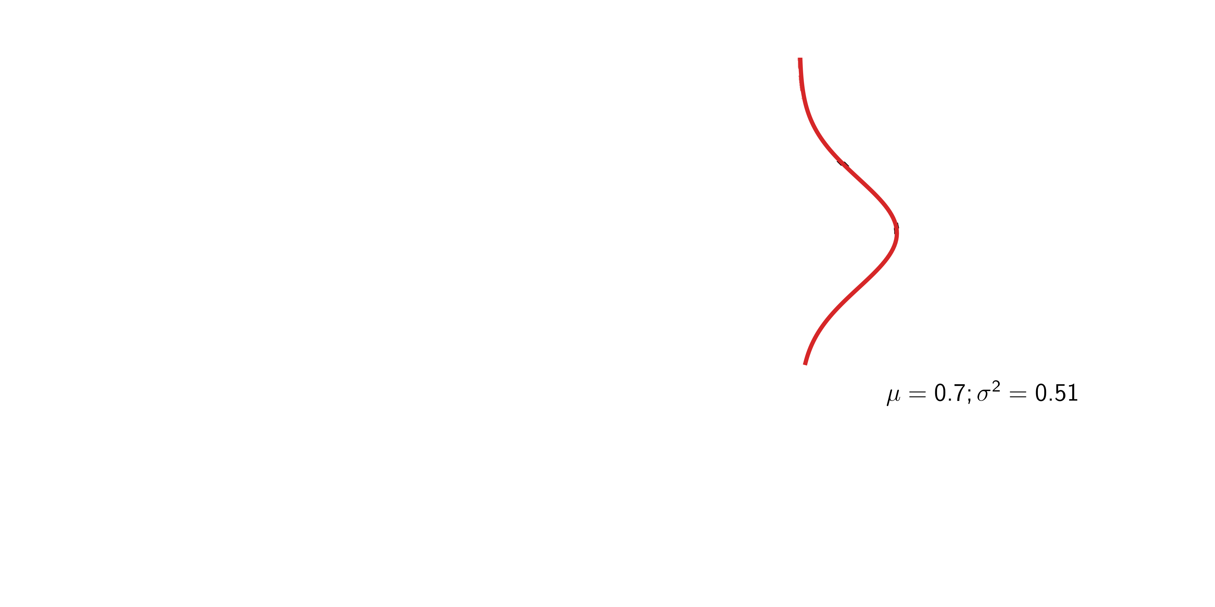
\[ \begin{aligned} p(x) &= \frac{1}{\sqrt{2\pi\sigma^2}}\exp\left(-\frac{(x - \mu)^2}{2\sigma^2}\right) % P(X \le x) &= \text{not known in closed form} \end{aligned} \]
If \(z \sim {\mathcal{N}}(0, 1)\), then \(x = \mu + \sigma z \sim {\mathcal{N}}(\mu, \sigma^2)\).
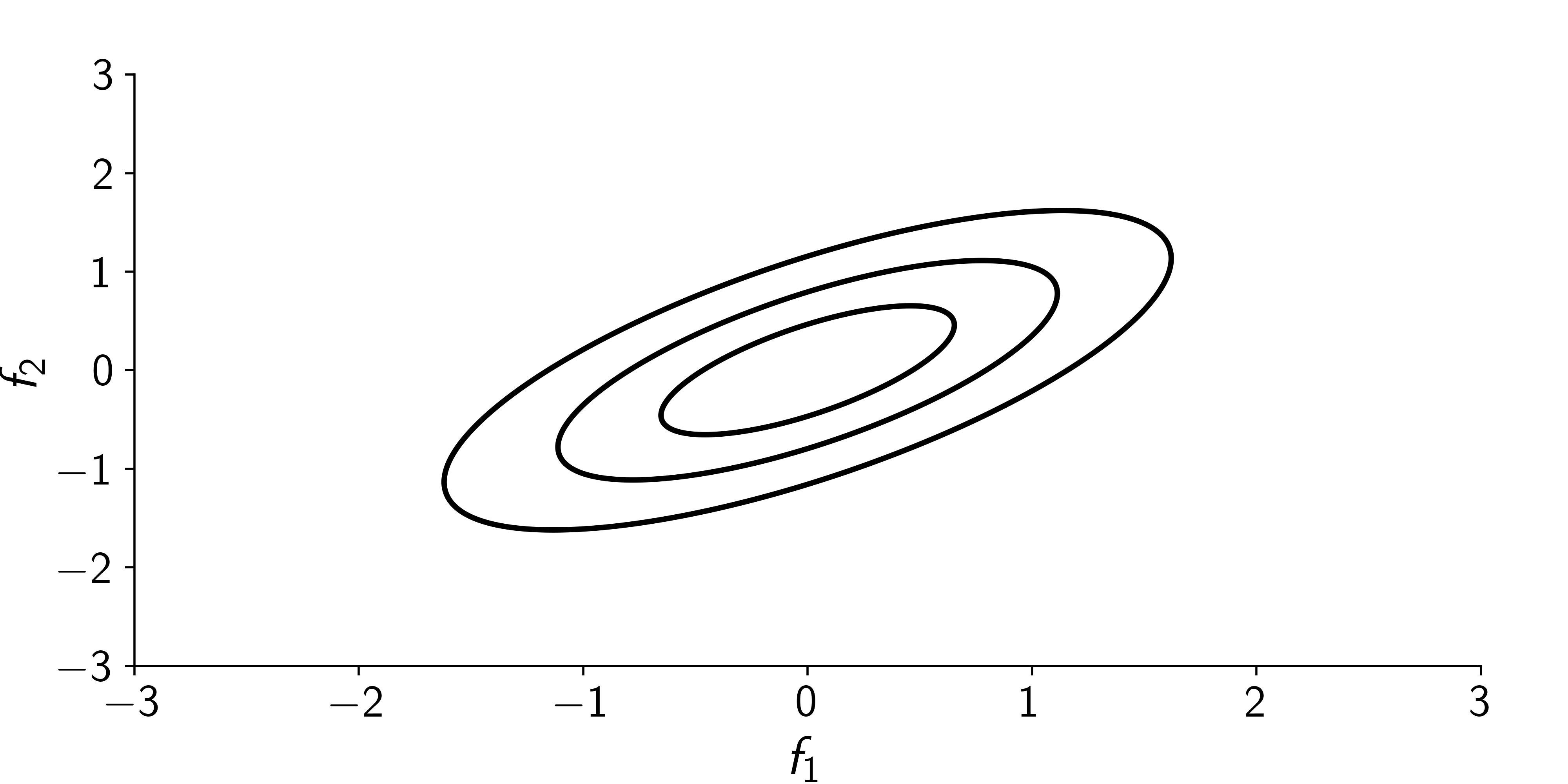
\[ {\boldsymbol{\mu}}= \begin{bmatrix} 0 \\ 0 \end{bmatrix} \quad {\boldsymbol{\Sigma}}= \begin{bmatrix} 1 & 0 \\ 0 & 1 \end{bmatrix} \]
\[ {\boldsymbol{\mu}}= \begin{bmatrix} 0 \\ 0 \end{bmatrix} \quad {\boldsymbol{\Sigma}}= \begin{bmatrix} 1 & 0 \\ 0 & 0.2 \end{bmatrix} \]
\[ {\boldsymbol{\mu}}= \begin{bmatrix} 0 \\ 0 \end{bmatrix} \quad {\boldsymbol{\Sigma}}= \begin{bmatrix} 1 & 0.7 \\ 0.7 & 1 \end{bmatrix} \]
\[ {\boldsymbol{\mu}}= \begin{bmatrix} 0 \\ 0 \end{bmatrix} \quad {\boldsymbol{\Sigma}}= \begin{bmatrix} 1 & 0.97 \\ 0.97 & 1 \end{bmatrix} \]
Gaussian distribution have several nice properties that make them attractive:
\[ {\textcolor{latent}{\boldsymbol{f}}}= \begin{bmatrix} {\textcolor{latent}{\boldsymbol{f}}}_1 \\ {\textcolor{latent}{\boldsymbol{f}}}_2 \end{bmatrix} \sim {\mathcal{N}}\left(\begin{bmatrix} {\boldsymbol{\mu}}_1 \\ {\boldsymbol{\mu}}_2 \end{bmatrix}, \begin{bmatrix} {\boldsymbol{\Sigma}}_{11} & {\boldsymbol{\Sigma}}_{12} \\ {\boldsymbol{\Sigma}}_{21} & {\boldsymbol{\Sigma}}_{22} \end{bmatrix}\right) \]
Then
\[ p({\textcolor{latent}{\boldsymbol{f}}}_2\mid{\textcolor{latent}{\boldsymbol{f}}}_1) = {\mathcal{N}}({\boldsymbol{\mu}}_2 + {\boldsymbol{\Sigma}}_{21}{\boldsymbol{\Sigma}}_{11}^{-1}({\textcolor{latent}{\boldsymbol{f}}}_1 - {\boldsymbol{\mu}}_1), {\boldsymbol{\Sigma}}_{22} - {\boldsymbol{\Sigma}}_{21}{\boldsymbol{\Sigma}}_{11}^{-1}{\boldsymbol{\Sigma}}_{12}) \]
which simplifies if \({\boldsymbol{\mu}}_1, {\boldsymbol{\mu}}_2 = {\boldsymbol{0}}\),
\[ p({\textcolor{latent}{\boldsymbol{f}}}_2\mid{\textcolor{latent}{\boldsymbol{f}}}_1) = {\mathcal{N}}({\boldsymbol{\Sigma}}_{21}{\boldsymbol{\Sigma}}_{11}^{-1}{\textcolor{latent}{\boldsymbol{f}}}_1, {\boldsymbol{\Sigma}}_{22} - {\boldsymbol{\Sigma}}_{21}{\boldsymbol{\Sigma}}_{11}^{-1}{\boldsymbol{\Sigma}}_{12}) \]
Tip
This is sometimes referred to as the Bayes’ rule for Gaussian distributions.
Hard to visualize in dimensions > 2, so let’s stack points next to each other.
So in 2D instead of: \(\qquad\qquad\qquad\qquad\qquad\qquad\qquad\) we have:
Consider \(D=5\) with
\[ \scriptsize {\boldsymbol{\mu}}= {\boldsymbol{0}}\qquad {\boldsymbol{\Sigma}}= \begin{bmatrix} 1 & 0.99 & 0.98 & 0.95 & 0.92 \\ 0.99 & 1 & 0.99 & 0.98 & 0.95 \\ 0.98 & 0.99 & 1 & 0.99 & 0.98 \\ 0.95 & 0.98 & 0.99 & 1 & 0.99 \\ 0.92 & 0.95 & 0.98 & 0.99 & 1 \end{bmatrix} \]
Consider \(D=50\) with
\[ \scriptsize {\boldsymbol{\mu}}= {\boldsymbol{0}}\qquad {\boldsymbol{\Sigma}}= \begin{bmatrix} 1 & 0.99 & 0.98 & \cdots \\ 0.99 & 1 & 0.99 & \cdots \\ 0.98 & 0.99 & 1 & \cdots \\ \vdots & \vdots & \vdots & \ddots \end{bmatrix} \]
We can think of a Gaussian process as an infinite-dimensional generalization of a multivariate Gaussian distribution.
… or as an infinite-dimensional distribution over functions.
All we need to do is to change indexes
A stochastic process is a collection of random variables indexed by some variable \(\textcolor{input}{x}\in {\mathcal{X}}\).
\[ \{\textcolor{latent}{f}(\textcolor{input}{x}) : \textcolor{input}{x}\in {\mathcal{X}}\} \]
Usually \(\textcolor{latent}{f}(\textcolor{input}{x}) \in {\mathbb{R}}\) and \({\mathcal{X}}= {\mathbb{R}}^D\). So, \(\textcolor{latent}{f}: {\mathbb{R}}^D \to {\mathbb{R}}\).
For a set of inputs \({\textcolor{input}{\boldsymbol{X}}}= \{\textcolor{input}{x}_1, \ldots, \textcolor{input}{x}_N\}\), the corresponding random variables \(\{\textcolor{latent}{f}_1, \ldots, \textcolor{latent}{f}_N\}\) with \(\textcolor{latent}{f}_i = \textcolor{latent}{f}(\textcolor{input}{x}_i)\) have a joint distribution \(p(\textcolor{latent}{f}(\textcolor{input}{x}_1), \ldots, \textcolor{latent}{f}(\textcolor{input}{x}_N))\).
A Gaussian process is a stochastic process such that any finite subset of the random variables has a joint Gaussian distribution.
\[ (\textcolor{latent}{f}(\textcolor{input}{x}_1), \ldots, \textcolor{latent}{f}(\textcolor{input}{x}_N)) \sim {\mathcal{N}}({\boldsymbol{\mu}}, {\boldsymbol{\Sigma}}) \]
We write \(\textcolor{latent}{f}\sim \mathcal{GP}\) to denote that \(\textcolor{latent}{f}\) is a Gaussian process.
To specify a Gaussian distribution, we need to define a mean vector \({\boldsymbol{\mu}}\) and a covariance matrix \({\boldsymbol{\Sigma}}\).
\[ {\boldsymbol{z}}\sim {\mathcal{N}}({\boldsymbol{\mu}}, {\boldsymbol{\Sigma}}) \]
To specify a Gaussian process, we need to define a mean function \(\mu(\textcolor{input}{x})\) and a covariance function \(k(\textcolor{input}{x}, \textcolor{input}{x}^\prime)\).
\[ f \sim \mathcal{GP}(\mu(\cdot), k(\cdot, \cdot)) \]
Take two points \(\textcolor{input}{x}_0\) and \(\textcolor{input}{x}_1\), their function values \(\textcolor{latent}{f}_0 = f(\textcolor{input}{x}_0)\) and \(\textcolor{latent}{f}_1 = f(\textcolor{input}{x}_1)\) are jointly Gaussian distributed with \(p(\textcolor{latent}{f}_0, \textcolor{latent}{f}_1)\).
We are free to choose the mean and the covariance functions however we like, subject to some constraints.
The mean function can be used to encode prior knowledge about the mean of the function we are trying to model.
The mean function \(\mu({\textcolor{input}{\boldsymbol{x}}})\) is often set to zero or constant.
The covariance function \(k({\textcolor{input}{\boldsymbol{x}}}, {\textcolor{input}{\boldsymbol{x}}}^\prime)\) is also known as the kernel function.
The covariance function encodes our prior beliefs about the family of functions we are trying to model.
Requirements for a valid covariance function:
We often assume \(k\) is a function of the difference between the inputs: \(k({\textcolor{input}{\boldsymbol{x}}}, {\textcolor{input}{\boldsymbol{x}}}^\prime) = k({\textcolor{input}{\boldsymbol{x}}}- {\textcolor{input}{\boldsymbol{x}}}^\prime)\), which is known as a stationary kernel.
RBF kernel or squared exponential kernel:
\[ k({\textcolor{input}{\boldsymbol{x}}}, {\textcolor{input}{\boldsymbol{x}}}^\prime) = \textcolor{vparams}\alpha \exp\left(-\frac{1}{2\textcolor{vparams}\lambda^2}({\textcolor{input}{\boldsymbol{x}}}- {\textcolor{input}{\boldsymbol{x}}}^\prime)^\top({\textcolor{input}{\boldsymbol{x}}}- {\textcolor{input}{\boldsymbol{x}}}^\prime)\right) = \textcolor{vparams}\alpha \exp\left(-\frac{1}{2\textcolor{vparams}\lambda^2}\norm{{\textcolor{input}{\boldsymbol{x}}}- {\textcolor{input}{\boldsymbol{x}}}^\prime}^2\right) \]
Defines smooth functions, where the function values are highly correlated for nearby inputs.
Hyperparameters:
\[ k({\textcolor{input}{\boldsymbol{x}}}, {\textcolor{input}{\boldsymbol{x}}}^\prime) = \textcolor{vparams}1 \exp\left(-\frac{1}{2\cdot\textcolor{vparams}1^2}\norm{{\textcolor{input}{\boldsymbol{x}}}- {\textcolor{input}{\boldsymbol{x}}}^\prime}^2\right) \]
\[ k({\textcolor{input}{\boldsymbol{x}}}, {\textcolor{input}{\boldsymbol{x}}}^\prime) = \textcolor{vparams}1 \exp\left(-\frac{1}{2\cdot\textcolor{vparams}{0.25}^2}\norm{{\textcolor{input}{\boldsymbol{x}}}- {\textcolor{input}{\boldsymbol{x}}}^\prime}^2\right) \]
\[ k({\textcolor{input}{\boldsymbol{x}}}, {\textcolor{input}{\boldsymbol{x}}}^\prime) = \textcolor{vparams}1 \exp\left(-\frac{1}{2\cdot\textcolor{vparams}{4}^2}\norm{{\textcolor{input}{\boldsymbol{x}}}- {\textcolor{input}{\boldsymbol{x}}}^\prime}^2\right) \]
\[ k({\textcolor{input}{\boldsymbol{x}}}, {\textcolor{input}{\boldsymbol{x}}}^\prime) = \textcolor{vparams}{10} \exp\left(-\frac{1}{2\cdot\textcolor{vparams}{1}^2}\norm{{\textcolor{input}{\boldsymbol{x}}}- {\textcolor{input}{\boldsymbol{x}}}^\prime}^2\right) \]
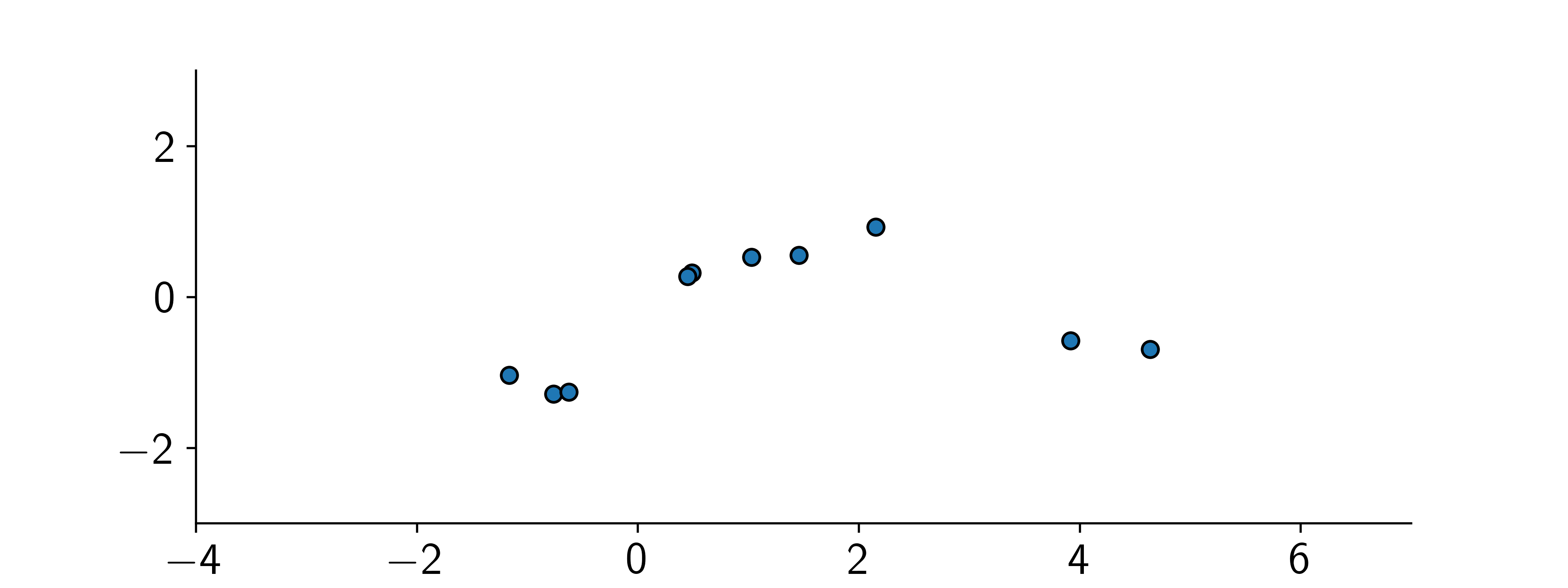
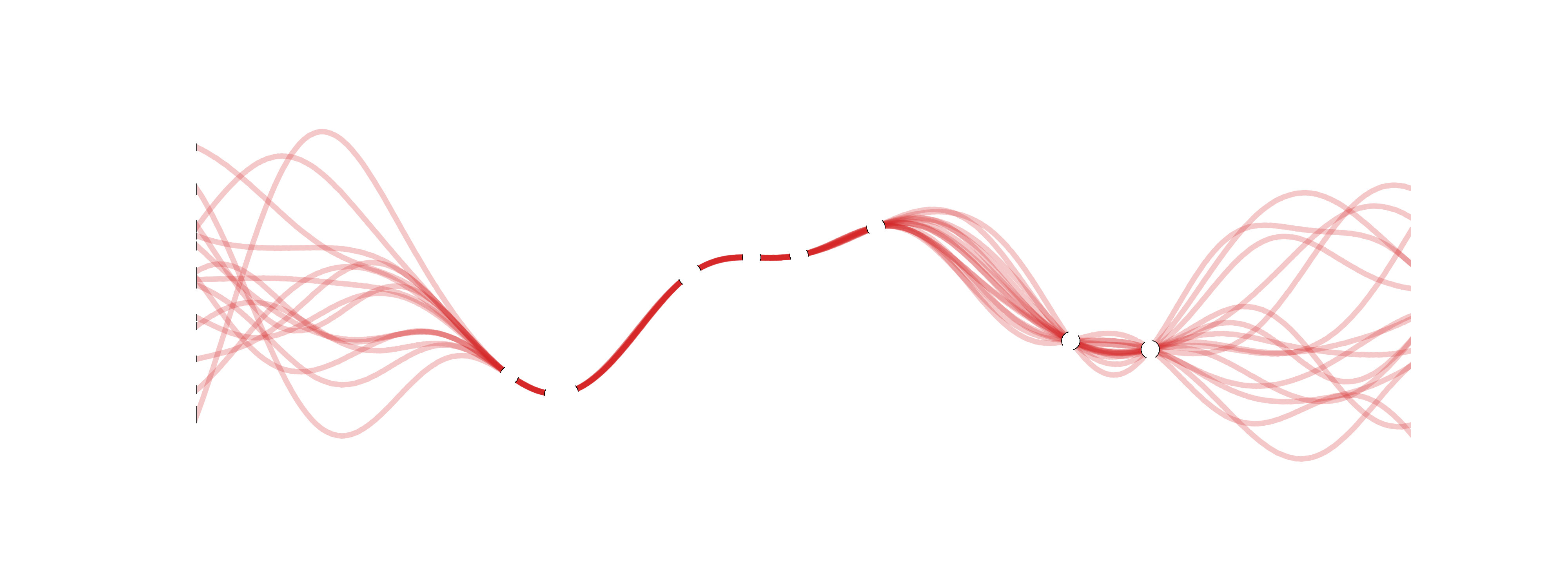
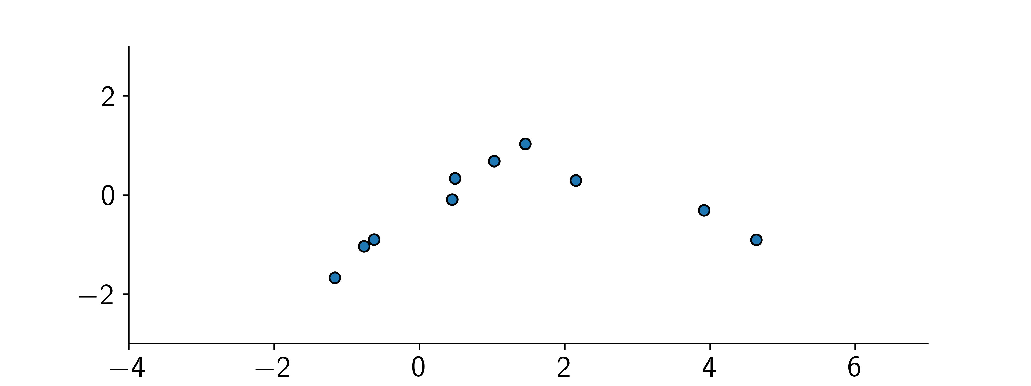
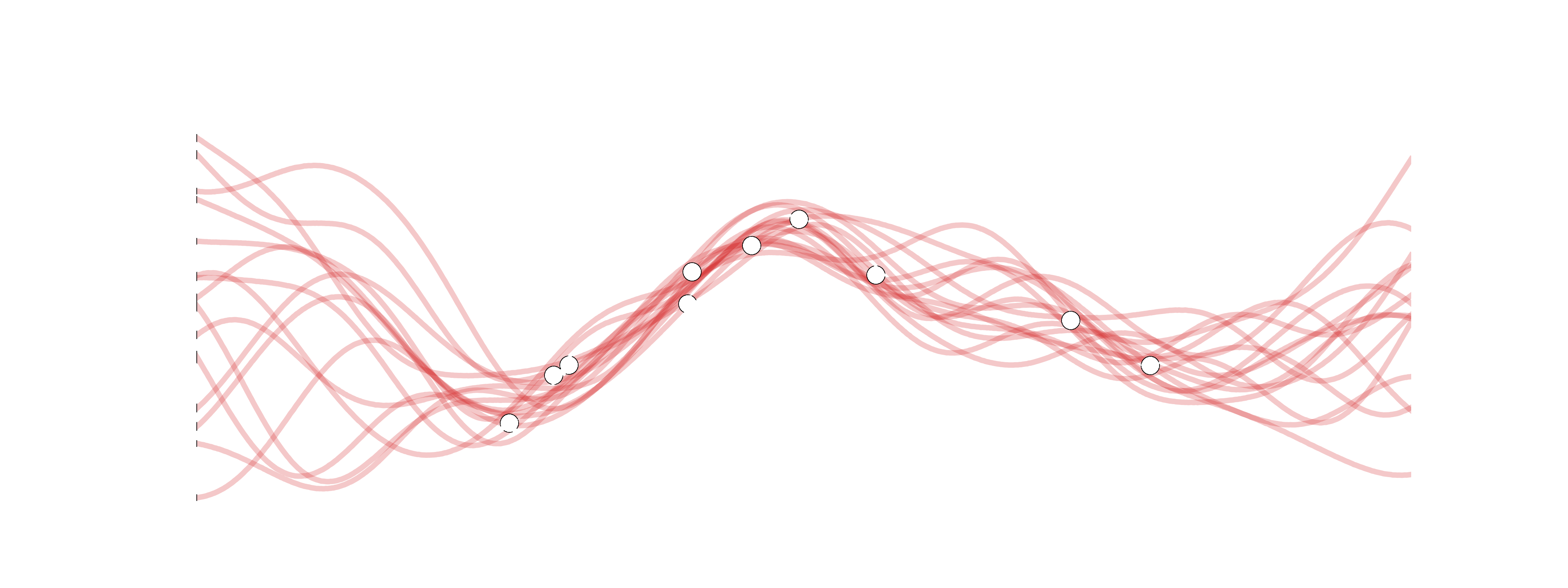
Given a set of training inputs \({\textcolor{input}{\boldsymbol{X}}}=\{{\textcolor{input}{\boldsymbol{x}}}_1, \ldots, {\textcolor{input}{\boldsymbol{x}}}_N\}\) and outputs \({\textcolor{latent}{\boldsymbol{f}}}=\{\textcolor{latent}{f}_1, \ldots, \textcolor{latent}{f}_N\}\), we want to make predictions for a new input \({\textcolor{input}{\boldsymbol{x}}}_\star\).
The joint distribution of the training outputs \({\textcolor{latent}{\boldsymbol{f}}}\) and the test output \(\textcolor{latent}{f}_\star\) is Gaussian:
\[ \begin{bmatrix} {\textcolor{latent}{\boldsymbol{f}}}\\ \textcolor{latent}{f}_\star \end{bmatrix} \sim {\mathcal{N}}\left({\boldsymbol{0}}, \begin{bmatrix} {\boldsymbol{K}}& {\boldsymbol{k}}_\star \\ {\boldsymbol{k}}_\star^\top & k_{\star\star} \end{bmatrix}\right) \]
where \({\boldsymbol{K}}=k({\textcolor{input}{\boldsymbol{X}}}, {\textcolor{input}{\boldsymbol{X}}})\), \({\boldsymbol{k}}_\star=k({\textcolor{input}{\boldsymbol{X}}}, {\textcolor{input}{\boldsymbol{x}}}_\star)\), and \(k_{\star\star}=k({\textcolor{input}{\boldsymbol{x}}}_\star, {\textcolor{input}{\boldsymbol{x}}}_\star)\).
Because of the Gaussian conditioning property, the distribution of \(\textcolor{latent}{f}_\star\) given \({\textcolor{latent}{\boldsymbol{f}}}\) is also Gaussian:
\[ \textcolor{latent}{f}_\star \mid {\textcolor{latent}{\boldsymbol{f}}}\sim {\mathcal{N}}({\boldsymbol{k}}_\star^\top{\boldsymbol{K}}^{-1}{\textcolor{latent}{\boldsymbol{f}}}, k_{\star\star} - {\boldsymbol{k}}_\star^\top{\boldsymbol{K}}^{-1}{\boldsymbol{k}}_\star) \]
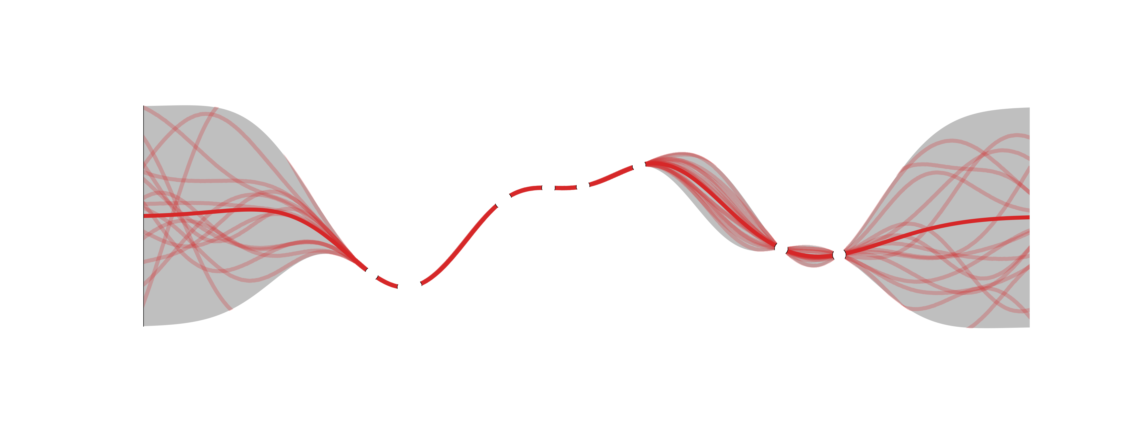
\[ \textcolor{latent}{f}_\star \mid {\textcolor{latent}{\boldsymbol{f}}}\sim {\mathcal{N}}({\boldsymbol{k}}_\star^\top{\boldsymbol{K}}^{-1}{\textcolor{latent}{\boldsymbol{f}}}, k_{\star\star} - {\boldsymbol{k}}_\star^\top{\boldsymbol{K}}^{-1}{\boldsymbol{k}}_\star) \]
Assumes that the training outputs \({\textcolor{latent}{\boldsymbol{f}}}\) are noise-free. This is not the assumption we made previously.
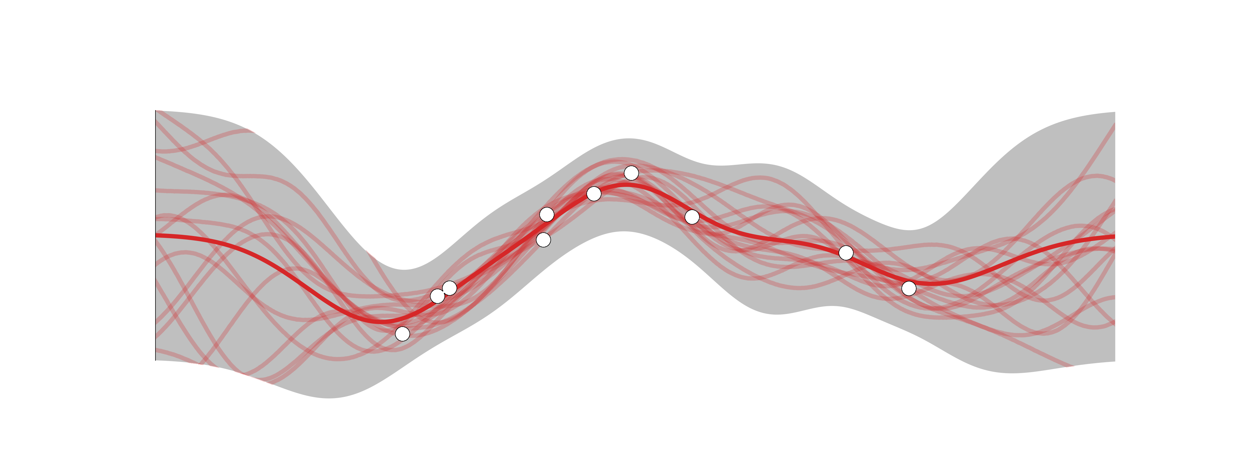
In general, we model the noise in the outputs as: \[ p({\textcolor{output}{\boldsymbol{y}}}\mid {\textcolor{latent}{\boldsymbol{f}}}) = {\mathcal{N}}({\textcolor{output}{\boldsymbol{y}}}\mid {\textcolor{latent}{\boldsymbol{f}}}, \sigma^2{\boldsymbol{I}}) \]
The joint distribution of the training outputs \({\textcolor{output}{\boldsymbol{y}}}\) and the test output \(\textcolor{latent}{f}_\star\) is still Gaussian, but with an additional noise term:
\[ \begin{bmatrix} {\textcolor{output}{\boldsymbol{y}}}\\ \textcolor{latent}{f}_\star \end{bmatrix} \sim {\mathcal{N}}\left({\boldsymbol{0}}, \begin{bmatrix} {\boldsymbol{K}}+ \sigma^2{\boldsymbol{I}}& {\boldsymbol{k}}_\star \\ {\boldsymbol{k}}_\star^\top & k_{\star\star} \end{bmatrix}\right) \]
The distribution of \(\textcolor{latent}{f}_\star\) given \({\textcolor{output}{\boldsymbol{y}}}\) is:
\[ \textcolor{latent}{f}_\star \mid {\textcolor{output}{\boldsymbol{y}}}\sim {\mathcal{N}}({\boldsymbol{k}}_\star^\top({\boldsymbol{K}}+ \sigma^2{\boldsymbol{I}})^{-1}{\textcolor{output}{\boldsymbol{y}}}, k_{\star\star} - {\boldsymbol{k}}_\star^\top({\boldsymbol{K}}+ \sigma^2{\boldsymbol{I}})^{-1}{\boldsymbol{k}}_\star) \]
We can also marginalize out the noise to get the distribution of \(\textcolor{output}{y}_\star\):
\[ \textcolor{output}{y}_\star \mid {\textcolor{output}{\boldsymbol{y}}}\sim {\mathcal{N}}({\boldsymbol{k}}_\star^\top({\boldsymbol{K}}+ \sigma^2{\boldsymbol{I}})^{-1}{\textcolor{output}{\boldsymbol{y}}}, k_{\star\star} - {\boldsymbol{k}}_\star^\top({\boldsymbol{K}}+ \sigma^2{\boldsymbol{I}})^{-1}{\boldsymbol{k}}_\star+ \sigma^2) \]
Recall lecture on Bayesian Linear Regression:
\[ p({\textcolor{output}{\boldsymbol{y}}}\mid {\textcolor{params}{\boldsymbol{w}}}, {\textcolor{input}{\boldsymbol{X}}}) = {\mathcal{N}}({\textcolor{output}{\boldsymbol{y}}}\mid {\textcolor{input}{\boldsymbol{X}}}{\textcolor{params}{\boldsymbol{w}}}, \sigma^2{\boldsymbol{I}}) \]
\[ p({\textcolor{params}{\boldsymbol{w}}}) = {\mathcal{N}}({\textcolor{params}{\boldsymbol{w}}}\mid {\boldsymbol{0}}, {\boldsymbol{I}}) \]
\[ p({\textcolor{params}{\boldsymbol{w}}}\mid {\textcolor{output}{\boldsymbol{y}}}, {\textcolor{input}{\boldsymbol{X}}}) = {\mathcal{N}}({\textcolor{params}{\boldsymbol{w}}}\mid {\boldsymbol{\mu}}, {\boldsymbol{\Sigma}}) \]
with \[ {\boldsymbol{\Sigma}}= \left(\frac{1}{\sigma^2}{\textcolor{input}{\boldsymbol{X}}}^\top{\textcolor{input}{\boldsymbol{X}}}+ {\boldsymbol{I}}\right)^{-1} \quad \text{and} \quad {\boldsymbol{\mu}}= \sigma^{-2}{\boldsymbol{\Sigma}}{\textcolor{input}{\boldsymbol{X}}}^\top{\textcolor{output}{\boldsymbol{y}}} \]
\[ p(\textcolor{output}{y}_\star \mid {\textcolor{input}{\boldsymbol{x}}}_\star, {\textcolor{output}{\boldsymbol{y}}}, {\textcolor{input}{\boldsymbol{X}}}) = {\mathcal{N}}(\textcolor{output}{y}_\star \mid {\boldsymbol{\mu}}^\top{\textcolor{input}{\boldsymbol{x}}}_\star, {\textcolor{input}{\boldsymbol{x}}}_\star^\top{\boldsymbol{\Sigma}}{\textcolor{input}{\boldsymbol{x}}}_\star + \sigma^2) \]
\[ {\textcolor{input}{\boldsymbol{x}}}\to {\boldsymbol{\phi}}({\textcolor{input}{\boldsymbol{x}}}) = \begin{bmatrix} \phi_1({\textcolor{input}{\boldsymbol{x}}}) & \cdots & \phi_D({\textcolor{input}{\boldsymbol{x}}}) \end{bmatrix}^\top \]
The functions \(\phi_d({\textcolor{input}{\boldsymbol{x}}})\) are known as basis functions.
Define:
\[ {\textcolor{input}{\boldsymbol{\Phi}}}= \begin{bmatrix} \phi_1(\textcolor{input}{x}_1) & \cdots & \phi_D(\textcolor{input}{x}_1) \\ \vdots & \ddots & \vdots \\ \phi_1(\textcolor{input}{x}_N) & \cdots & \phi_D(\textcolor{input}{x}_N) \end{bmatrix} \in \mathbb{R}^{N \times D} \]
Apply Bayesian linear regression to the transformed inputs:
\[ p({\textcolor{params}{\boldsymbol{w}}}\mid {\textcolor{output}{\boldsymbol{y}}}, {\textcolor{input}{\boldsymbol{X}}}) = {\mathcal{N}}({\textcolor{params}{\boldsymbol{w}}}\mid {\boldsymbol{\mu}}, {\boldsymbol{\Sigma}}) \]
where
\[ {\boldsymbol{\Sigma}}= \left(\frac{1}{\sigma^2}{\textcolor{input}{\boldsymbol{\Phi}}}^\top{\textcolor{input}{\boldsymbol{\Phi}}}+ {\boldsymbol{I}}\right)^{-1} \quad \text{and} \quad {\boldsymbol{\mu}}= \sigma^{-2}{\boldsymbol{\Sigma}}{\textcolor{input}{\boldsymbol{\Phi}}}^\top{\textcolor{output}{\boldsymbol{y}}} \]
\[ p(\textcolor{output}{y}_\star \mid {\textcolor{input}{\boldsymbol{x}}}_\star, {\textcolor{output}{\boldsymbol{y}}}, {\textcolor{input}{\boldsymbol{X}}}) = {\mathcal{N}}(\textcolor{output}{y}_\star \mid {\boldsymbol{\mu}}^\top\textcolor{input}{\boldsymbol{\phi}}_\star,\;\textcolor{input}{\boldsymbol{\phi}}_\star^\top{\boldsymbol{\Sigma}}\textcolor{input}{\boldsymbol{\phi}}_\star + \sigma^2) \]
where \(\textcolor{input}{\boldsymbol{\phi}}_\star = {\boldsymbol{\phi}}({\textcolor{input}{\boldsymbol{x}}}_\star)\).
\[ k({\textcolor{input}{\boldsymbol{x}}}, {\textcolor{input}{\boldsymbol{x}}}^\prime) = {\boldsymbol{\phi}}({\textcolor{input}{\boldsymbol{x}}})^\top{\boldsymbol{\phi}}({\textcolor{input}{\boldsymbol{x}}}^\prime) \]
This is known as the kernel trick.
The kernel function \(k({\textcolor{input}{\boldsymbol{x}}}, {\textcolor{input}{\boldsymbol{x}}}^\prime)\) is a measure of similarity between two inputs \({\textcolor{input}{\boldsymbol{x}}}\) and \({\textcolor{input}{\boldsymbol{x}}}^\prime\).
For a matrix input \({\textcolor{input}{\boldsymbol{X}}}\), the kernel matrix is defined as
\[ {\boldsymbol{K}}= {\textcolor{input}{\boldsymbol{\Phi}}}{\textcolor{input}{\boldsymbol{\Phi}}}^\top = \begin{bmatrix} k({\textcolor{input}{\boldsymbol{x}}}_1, {\textcolor{input}{\boldsymbol{x}}}_1) & \cdots & k({\textcolor{input}{\boldsymbol{x}}}_1, {\textcolor{input}{\boldsymbol{x}}}_N) \\ \vdots & \ddots & \vdots \\ k({\textcolor{input}{\boldsymbol{x}}}_N, {\textcolor{input}{\boldsymbol{x}}}_1) & \cdots & k({\textcolor{input}{\boldsymbol{x}}}_N, {\textcolor{input}{\boldsymbol{x}}}_N) \end{bmatrix} \in \mathbb{R}^{N \times N} \]
Woodbury matrix identity
Recall the Woodbury matrix identity: \[ ({\boldsymbol{A}}+ {\boldsymbol{U}}{\boldsymbol{C}}{\boldsymbol{V}})^{-1} = {\boldsymbol{A}}^{-1} - {\boldsymbol{A}}^{-1}{\boldsymbol{U}}({\boldsymbol{C}}^{-1} + {\boldsymbol{V}}{\boldsymbol{A}}^{-1}{\boldsymbol{U}})^{-1}{\boldsymbol{V}}{\boldsymbol{A}}^{-1} \] (Do not remember this formula!)
Use the Woodbury matrix identity to rewrite the posterior covariance:
\[ \begin{aligned} {\boldsymbol{\Sigma}}&= \left(\frac{1}{\sigma^2}{\textcolor{input}{\boldsymbol{\Phi}}}^\top{\textcolor{input}{\boldsymbol{\Phi}}}+ {\boldsymbol{I}}\right)^{-1} \\ &= {\boldsymbol{I}}- {\textcolor{input}{\boldsymbol{\Phi}}}^\top\left(\sigma^2{\boldsymbol{I}}+ {\textcolor{input}{\boldsymbol{\Phi}}}{\textcolor{input}{\boldsymbol{\Phi}}}^\top\right)^{-1}{\textcolor{input}{\boldsymbol{\Phi}}} \end{aligned} \]
\[ p(\textcolor{output}{y}_\star \mid {\textcolor{input}{\boldsymbol{x}}}_\star, {\textcolor{output}{\boldsymbol{y}}}, {\textcolor{input}{\boldsymbol{X}}}) = {\mathcal{N}}(\textcolor{output}{y}_\star \mid {\boldsymbol{\mu}}^\top\textcolor{input}{\boldsymbol{\phi}}_\star,\;\textcolor{input}{\boldsymbol{\phi}}_\star^\top{\boldsymbol{\Sigma}}\textcolor{input}{\boldsymbol{\phi}}_\star + \sigma^2) \]
We want to express the predictive mean and variance in terms of scalar products of the basis functions.
Variance:
\[ \begin{aligned} \textcolor{input}{\boldsymbol{\phi}}_\star^\top{\boldsymbol{\Sigma}}\textcolor{input}{\boldsymbol{\phi}}_\star + \sigma^2 &= \textcolor{input}{\boldsymbol{\phi}}_\star^\top\left({\boldsymbol{I}}- {\textcolor{input}{\boldsymbol{\Phi}}}^\top\left(\sigma^2{\boldsymbol{I}}+ {\textcolor{input}{\boldsymbol{\Phi}}}{\textcolor{input}{\boldsymbol{\Phi}}}^\top\right)^{-1}{\textcolor{input}{\boldsymbol{\Phi}}}\right)\textcolor{input}{\boldsymbol{\phi}}_\star + \sigma^2 \\ &= \textcolor{input}{\boldsymbol{\phi}}_\star^\top\textcolor{input}{\boldsymbol{\phi}}_\star - \textcolor{input}{\boldsymbol{\phi}}_\star^\top{\textcolor{input}{\boldsymbol{\Phi}}}^\top\left(\sigma^2{\boldsymbol{I}}+ {\textcolor{input}{\boldsymbol{\Phi}}}{\textcolor{input}{\boldsymbol{\Phi}}}^\top\right)^{-1}{\textcolor{input}{\boldsymbol{\Phi}}}\textcolor{input}{\boldsymbol{\phi}}_\star + \sigma^2 \\ &= k_{\star\star} - {\boldsymbol{k}}_\star^\top({\boldsymbol{K}}+ \sigma^2{\boldsymbol{I}})^{-1}{\boldsymbol{k}}_\star + \sigma^2 \end{aligned} \]
where \({\boldsymbol{k}}_\star = k({\textcolor{input}{\boldsymbol{X}}}, {\textcolor{input}{\boldsymbol{x}}}_\star)\) and \(k_{\star\star} = k({\textcolor{input}{\boldsymbol{x}}}_\star, {\textcolor{input}{\boldsymbol{x}}}_\star)\).
Compare this with the predictive variance in the Gaussian process we have seen before.
Mean:
\[ \begin{aligned} {\boldsymbol{\mu}}^\top\textcolor{input}{\boldsymbol{\phi}}_\star &= \sigma^{-2}\textcolor{input}{\boldsymbol{\phi}}_\star^\top{\boldsymbol{\Sigma}}{\textcolor{input}{\boldsymbol{\Phi}}}^\top{\textcolor{output}{\boldsymbol{y}}}\\ &= \sigma^{-2}\textcolor{input}{\boldsymbol{\phi}}_\star^\top\left({\boldsymbol{I}}- {\textcolor{input}{\boldsymbol{\Phi}}}^\top\left(\sigma^2{\boldsymbol{I}}+ {\textcolor{input}{\boldsymbol{\Phi}}}{\textcolor{input}{\boldsymbol{\Phi}}}^\top\right)^{-1}{\textcolor{input}{\boldsymbol{\Phi}}}\right){\textcolor{input}{\boldsymbol{\Phi}}}^\top{\textcolor{output}{\boldsymbol{y}}}\\ &= \sigma^{-2}\textcolor{input}{\boldsymbol{\phi}}_\star^\top {\textcolor{input}{\boldsymbol{\Phi}}}^\top \left( {\boldsymbol{I}}- \left(\sigma^2{\boldsymbol{I}}+ {\textcolor{input}{\boldsymbol{\Phi}}}{\textcolor{input}{\boldsymbol{\Phi}}}^\top\right)^{-1}{\textcolor{input}{\boldsymbol{\Phi}}}{\textcolor{input}{\boldsymbol{\Phi}}}^\top \right){\textcolor{output}{\boldsymbol{y}}}\\ &= \sigma^{-2}\textcolor{input}{\boldsymbol{\phi}}_\star^\top {\textcolor{input}{\boldsymbol{\Phi}}}^\top \left( {\boldsymbol{I}}- \left({\boldsymbol{I}}+ \sigma^{-2}{\textcolor{input}{\boldsymbol{\Phi}}}{\textcolor{input}{\boldsymbol{\Phi}}}^\top\right)^{-1}\sigma^{-2}{\textcolor{input}{\boldsymbol{\Phi}}}{\textcolor{input}{\boldsymbol{\Phi}}}^\top \right){\textcolor{output}{\boldsymbol{y}}}\\ \end{aligned} \]
Apply again the Woodbury matrix identity with \({\boldsymbol{A}},{\boldsymbol{U}},{\boldsymbol{V}}= {\boldsymbol{I}}\) and \({\boldsymbol{C}}= \left(\sigma^{-2}{\textcolor{input}{\boldsymbol{\Phi}}}{\textcolor{input}{\boldsymbol{\Phi}}}^\top\right)^{-1}\):
\[ {\boldsymbol{I}}- \left({\boldsymbol{I}}+ \sigma^{-2}{\textcolor{input}{\boldsymbol{\Phi}}}{\textcolor{input}{\boldsymbol{\Phi}}}^\top\right)^{-1}\sigma^{-2}{\textcolor{input}{\boldsymbol{\Phi}}}{\textcolor{input}{\boldsymbol{\Phi}}}^\top = \left( {\boldsymbol{I}}+ \sigma^{-2}{\textcolor{input}{\boldsymbol{\Phi}}}{\textcolor{input}{\boldsymbol{\Phi}}}^\top \right)^{-1} \]
continue…
\[ \begin{aligned} {\boldsymbol{\mu}}^\top\textcolor{input}{\boldsymbol{\phi}}_\star &= \sigma^{-2}\textcolor{input}{\boldsymbol{\phi}}_\star^\top {\textcolor{input}{\boldsymbol{\Phi}}}^\top \left( {\boldsymbol{I}}- \left({\boldsymbol{I}}+ \sigma^{-2}{\textcolor{input}{\boldsymbol{\Phi}}}{\textcolor{input}{\boldsymbol{\Phi}}}^\top\right)^{-1}\sigma^{-2}{\textcolor{input}{\boldsymbol{\Phi}}}{\textcolor{input}{\boldsymbol{\Phi}}}^\top \right){\textcolor{output}{\boldsymbol{y}}}\\ &= \sigma^{-2}\textcolor{input}{\boldsymbol{\phi}}_\star^\top {\textcolor{input}{\boldsymbol{\Phi}}}^\top \left( {\boldsymbol{I}}+ \sigma^{-2}{\textcolor{input}{\boldsymbol{\Phi}}}{\textcolor{input}{\boldsymbol{\Phi}}}^\top \right)^{-1}{\textcolor{output}{\boldsymbol{y}}}\\ &= \textcolor{input}{\boldsymbol{\phi}}_\star^\top {\textcolor{input}{\boldsymbol{\Phi}}}^\top \left( \sigma^2{\boldsymbol{I}}+ {\textcolor{input}{\boldsymbol{\Phi}}}{\textcolor{input}{\boldsymbol{\Phi}}}^\top \right)^{-1}{\textcolor{output}{\boldsymbol{y}}}\\ &= {\boldsymbol{k}}_\star^\top({\boldsymbol{K}}+ \sigma^2{\boldsymbol{I}})^{-1}{\textcolor{output}{\boldsymbol{y}}} \end{aligned} \]
Again, compare this with the predictive mean in the Gaussian process we have seen before.
You can either to linear regression by working with the feature mappings \({\boldsymbol{\phi}}(\cdot)\) or with the kernel function \(k(\cdot, \cdot)\).
If \(D \gg N\), the kernel trick is more efficient.
For example, working with \(k(\cdot, \cdot)\) allows us to implicitly use infinite-dimensional feature spaces.
One of such examples is the RBF (or squared exponential) kernel we have seen before:
\[ k({\textcolor{input}{\boldsymbol{x}}}, {\textcolor{input}{\boldsymbol{x}}}^\prime) = \textcolor{vparams}\alpha \exp\left(-\frac{1}{2\textcolor{vparams}\lambda^2}\norm{{\textcolor{input}{\boldsymbol{x}}}- {\textcolor{input}{\boldsymbol{x}}}^\prime}^2\right) \]
We can show that the RBF kernel corresponds to an infinite-dimensional feature space.
Suppose \(\textcolor{vparams}\lambda = 1\) and \(\textcolor{vparams}\alpha = 1\), and \({\textcolor{input}{\boldsymbol{x}}}\in {\mathbb{R}}\).
\[ k(\textcolor{input}{x}, \textcolor{input}{x}^\prime) = \exp\left(-\frac{1}{2}(\textcolor{input}{x}- \textcolor{input}{x}^\prime)^2\right) = \exp\left(-\frac{1}{2}\textcolor{input}{x}^2\right)\exp\left(-\frac{1}{2}{\textcolor{input}{x}^\prime}^2\right)\exp(\textcolor{input}{x}\textcolor{input}{x}^\prime) \]
Use the Taylor expansion of the exponential function:
\[ \exp(\textcolor{input}{x}\textcolor{input}{x}^\prime) = 1 + \textcolor{input}{x}\textcolor{input}{x}^\prime + \frac{1}{2!}(\textcolor{input}{x}\textcolor{input}{x}^\prime)^2 + \frac{1}{3!}(\textcolor{input}{x}\textcolor{input}{x}^\prime)^3 + \cdots \]
Define the infinite-dimensional feature mappings:
\[ \textcolor{input}{x}\to \phi(\textcolor{input}{x}) = \exp\left(-\frac{1}{2}\textcolor{input}{x}^2\right)\begin{bmatrix} 1 & \textcolor{input}{x}& \frac{1}{\sqrt{2!}}\textcolor{input}{x}^2 & \frac{1}{\sqrt{3!}}\textcolor{input}{x}^3 & \cdots \end{bmatrix}^\top \]
In practice, we need to choose the kernel function and its hyperparameters.
The choice of the kernel function and its hyperparameters is known as model selection.
We already saw how to do model selection in Bayesian linear regression using the marginal likelihood.
In Gaussian processes, we can also use the marginal likelihood to perform model selection.
\[ p({\textcolor{output}{\boldsymbol{y}}}) = \int p({\textcolor{output}{\boldsymbol{y}}}\mid {\textcolor{latent}{\boldsymbol{f}}})p({\textcolor{latent}{\boldsymbol{f}}}) \dd{\textcolor{latent}{\boldsymbol{f}}} \]
Let’s be explicit about the hyperparameters \({\textcolor{params}{\boldsymbol{\theta}}}\) of the kernel function \(k(\cdot, \cdot)\): \[ p({\textcolor{output}{\boldsymbol{y}}}\mid {\textcolor{params}{\boldsymbol{\theta}}}) = \int p({\textcolor{output}{\boldsymbol{y}}}\mid {\textcolor{latent}{\boldsymbol{f}}}, {\textcolor{params}{\boldsymbol{\theta}}})p({\textcolor{latent}{\boldsymbol{f}}}\mid {\textcolor{params}{\boldsymbol{\theta}}}) \dd{\textcolor{latent}{\boldsymbol{f}}}= {\mathcal{N}}({\textcolor{output}{\boldsymbol{y}}}\mid {\boldsymbol{0}}, {\boldsymbol{K}}+ \sigma^2{\boldsymbol{I}}) \]
Maximize the marginal (log-)likelihood with respect to the hyperparameters \({\textcolor{params}{\boldsymbol{\theta}}}\):
\[ \arg\max_{{\textcolor{params}{\boldsymbol{\theta}}}} \log p({\textcolor{output}{\boldsymbol{y}}}\mid {\textcolor{params}{\boldsymbol{\theta}}}) = \arg\max_{{\textcolor{params}{\boldsymbol{\theta}}}} -\frac{1}{2}{\textcolor{output}{\boldsymbol{y}}}^\top({\boldsymbol{K}}+ \sigma^2{\boldsymbol{I}})^{-1}{\textcolor{output}{\boldsymbol{y}}}- \frac{1}{2}\log\det({\boldsymbol{K}}+ \sigma^2{\boldsymbol{I}}) - \frac{N}{2}\log(2\pi) \]
Question: How to optimize the marginal likelihood?
The marginal likelihood is a non-convex function of the hyperparameters \({\textcolor{params}{\boldsymbol{\theta}}}\).
No closed-form solution to the optimization problem, but we can use gradient-based optimization methods.
We can use automatic differentiation to compute the gradients of the marginal likelihood with respect to the hyperparameters.
\[ \frac{\partial}{\partial {\textcolor{params}{\boldsymbol{\theta}}}_i} \log p({\textcolor{output}{\boldsymbol{y}}}\mid {\textcolor{params}{\boldsymbol{\theta}}}) = \frac{1}{2}{\textcolor{output}{\boldsymbol{y}}}^\top({\boldsymbol{K}}+ \sigma^2{\boldsymbol{I}})^{-1}\frac{\partial {\boldsymbol{K}}}{\partial {\textcolor{params}{\boldsymbol{\theta}}}_i}({\boldsymbol{K}}+ \sigma^2{\boldsymbol{I}})^{-1}{\textcolor{output}{\boldsymbol{y}}}- \frac{1}{2}\text{tr}\left(({\boldsymbol{K}}+ \sigma^2{\boldsymbol{I}})^{-1}\frac{\partial {\boldsymbol{K}}}{\partial {\textcolor{params}{\boldsymbol{\theta}}}_i}\right) \]
Remember to guarantee that the hyperparameters are valid (e.g., positive for the length scale).
\[ \underbrace{- \frac{1}{2} {\textcolor{output}{\boldsymbol{y}}}^\top ({\boldsymbol{K}}+ \sigma^2{\boldsymbol{I}})^{-1} {\textcolor{output}{\boldsymbol{y}}}}_{\text{Model fit}} - \frac{1}{2} \underbrace{\log \det({\boldsymbol{K}}+ \sigma^2{\boldsymbol{I}})}_{\text{Model complexity}} - \frac{N}{2} \log(2\pi) \]
The marginal likelihood is a trade-off between the fit to the data and the complexity of the model.
Problem of non-idenditifiability: multiple configurations of the hyperparameters can lead to the similar marginal likelihood.
Non-Gaussian likelihoods: Gaussian processes assume Gaussian likelihoods, but many real-world datasets have non-Gaussian likelihoods.
Scalability: Gaussian processes have \(\mathcal O(N^3)\) complexity in the number of data points \(N\).
Non-stationary kernels: Many real-world datasets have non-stationary patterns that are not well captured by stationary kernels.
Model the latent function \(f({\textcolor{input}{\boldsymbol{x}}})\) as a Gaussian process and apply sigmoid function to get the probability of the class label: \[ p(\textcolor{output}{y}=1 \mid {\textcolor{input}{\boldsymbol{x}}}) = \sigma(f({\textcolor{input}{\boldsymbol{x}}})) \]
Equivalent to assume the Bernoulli likelihood… \[ p(\textcolor{output}{y}\mid \textcolor{latent}{f}) = \text{Bern}(\textcolor{output}{y}\mid \sigma(\textcolor{latent}{f})) \]
… and factorization \[ p({\textcolor{output}{\boldsymbol{y}}}\mid {\textcolor{latent}{\boldsymbol{f}}}) = \prod_{n=1}^N p(\textcolor{output}{y}_n \mid \textcolor{latent}{f}_n) \]
The posterior predictive distribution is not Gaussian anymore and intractable.
\[ p(\textcolor{latent}{f}_\star \mid {\textcolor{output}{\boldsymbol{y}}}) = \int p(\textcolor{latent}{f}_\star \mid {\textcolor{latent}{\boldsymbol{f}}})p({\textcolor{latent}{\boldsymbol{f}}}\mid{\textcolor{output}{\boldsymbol{y}}}) \dd{\textcolor{latent}{\boldsymbol{f}}} \]
where \(p({\textcolor{latent}{\boldsymbol{f}}}\mid{\textcolor{output}{\boldsymbol{y}}}) = p({\textcolor{output}{\boldsymbol{y}}}\mid{\textcolor{latent}{\boldsymbol{f}}})p({\textcolor{latent}{\boldsymbol{f}}})/p({\textcolor{output}{\boldsymbol{y}}})\) is the posterior distribution of the functions given the data.
\[ p(\textcolor{output}{y}_\star = 1 \mid {\textcolor{output}{\boldsymbol{y}}}) = \int \sigma(\textcolor{latent}{f}_\star) p(\textcolor{latent}{f}_\star \mid {\textcolor{output}{\boldsymbol{y}}}) \dd{\textcolor{latent}{f}_\star} \]
where \(\sigma(\cdot)\) is the sigmoid function.
As we did for Bayesian logistic regression, we need to use approximate inference methods.
Laplace approximation:
Variational inferece
Objective: Approximate \(p({\textcolor{latent}{\boldsymbol{f}}}\mid {\textcolor{output}{\boldsymbol{y}}})\) as a Gaussian distribution \(q({\textcolor{latent}{\boldsymbol{f}}}) = {\mathcal{N}}({\textcolor{latent}{\boldsymbol{f}}}\mid \widehat{\textcolor{latent}{\boldsymbol{f}}}, {\boldsymbol{H}}^{-1})\).
Write the (log) posterior distribution as:
\[ \begin{aligned} {\mathcal{L}}({\textcolor{latent}{\boldsymbol{f}}}) &= \log p({\textcolor{output}{\boldsymbol{y}}}\mid {\textcolor{latent}{\boldsymbol{f}}}) + \log p({\textcolor{latent}{\boldsymbol{f}}}) = \log p({\textcolor{output}{\boldsymbol{y}}}\mid {\textcolor{latent}{\boldsymbol{f}}}) - \frac{1}{2}{\textcolor{latent}{\boldsymbol{f}}}^\top{\boldsymbol{K}}^{-1}{\textcolor{latent}{\boldsymbol{f}}}- \frac{1}{2}\log\det{\boldsymbol{K}}- \frac{N}{2}\log(2\pi) \end{aligned} \]
Find the mode of the posterior distribution and use it as the mean of the Gaussian approximation. \[ \widehat{{\textcolor{latent}{\boldsymbol{f}}}} = \arg\max_{{\textcolor{latent}{\boldsymbol{f}}}} {\mathcal{L}}({\textcolor{latent}{\boldsymbol{f}}}) \]
Compute the Hessian at the mode and use it as inverse covariance of the Gaussian approximation. \[ {\boldsymbol{H}}= \grad_{{\textcolor{latent}{\boldsymbol{f}}}}^2 {\mathcal{L}}(\widehat{\textcolor{latent}{\boldsymbol{f}}}) = \underbrace{\grad_{{\textcolor{latent}{\boldsymbol{f}}}}^2 \log p({\textcolor{output}{\boldsymbol{y}}}\mid \widehat{\textcolor{latent}{\boldsymbol{f}}})}_{{\boldsymbol{D}}} - {\boldsymbol{K}}^{-1} \]
Objective: Approximate \(q(\textcolor{latent}{f}_\star \mid {\textcolor{output}{\boldsymbol{y}}})=\int p(\textcolor{latent}{f}_\star \mid {\textcolor{latent}{\boldsymbol{f}}})q({\textcolor{latent}{\boldsymbol{f}}}) \dd{\textcolor{latent}{\boldsymbol{f}}}\)
\[ p(\textcolor{latent}{f}_\star \mid {\textcolor{latent}{\boldsymbol{f}}}) = {\mathcal{N}}(\textcolor{latent}{f}_\star \mid {\boldsymbol{k}}_{\star}^\top{\boldsymbol{K}}^{-1}{\textcolor{latent}{\boldsymbol{f}}}, k_{\star\star} - {\boldsymbol{k}}_{\star}^\top{\boldsymbol{K}}^{-1}{\boldsymbol{k}}_{\star}) \]
\(q({\textcolor{latent}{\boldsymbol{f}}})\) is Gaussian with mean \(\widehat{\textcolor{latent}{\boldsymbol{f}}}\) and covariance \({\boldsymbol{H}}^{-1}= ({\boldsymbol{D}}- {\boldsymbol{K}}^{-1})^{-1}\).
The predictive distribution is a Gaussian with mean \({\boldsymbol{\mu}}\) and covariance \({\boldsymbol{\Sigma}}\):
\[ \begin{aligned} {\boldsymbol{\mu}}&= {\boldsymbol{k}}_{\star}^\top{\boldsymbol{K}}^{-1}\widehat{\textcolor{latent}{\boldsymbol{f}}}\\ {\boldsymbol{\Sigma}} % &= k_{\star\star} - \mbk_{\star}^\top\mbK^{-1}\mbk_{\star} + \mbk_{\star}^\top\mbK^{-1}\mbH\mbK^{-1}\mbk_{\star} = \\ &= k_{\star\star} - {\boldsymbol{k}}_{\star}^\top\left({\boldsymbol{K}}+ {\boldsymbol{D}}^{-1}\right)^{-1}{\boldsymbol{k}}_{\star} \end{aligned} \]
Objective: Compute the predictive distribution for the class label \(\textcolor{output}{y}_\star\).
\[ \begin{aligned} p(\textcolor{output}{y}_\star = 1 \mid {\textcolor{output}{\boldsymbol{y}}}) &= \int \sigma(\textcolor{latent}{f}_\star) p(\textcolor{latent}{f}_\star \mid {\textcolor{output}{\boldsymbol{y}}}) \dd{\textcolor{latent}{f}_\star} \\ &= \int \sigma(\textcolor{latent}{f}_\star) {\mathcal{N}}(\textcolor{latent}{f}_\star \mid {\boldsymbol{\mu}}, {\boldsymbol{\Sigma}}) \dd{\textcolor{latent}{f}_\star} \end{aligned} \]
\[ p(\textcolor{output}{y}_\star = 1 \mid {\textcolor{output}{\boldsymbol{y}}}) \approx \frac{1}{S}\sum_{s=1}^S \sigma(\textcolor{latent}{f}_\star^{(s)}) \quad \text{where} \quad \textcolor{latent}{f}_\star^{(s)} \sim {\mathcal{N}}({\boldsymbol{\mu}}, {\boldsymbol{\Sigma}}) \]
Anywhere where you have a dynamical system that you want to model and predict:
In robotic control
For gradient-free optimization (Bayesian optimization)

![]()
Simone Rossi - Advanced Statistical Inference - EURECOM


