Introduction to deep generative models

Advanced Statistical Inference

Simone Rossi

EURECOM

Generative models

\[ \require{physics} \definecolor{input}{rgb}{0.42, 0.55, 0.74} \definecolor{params}{rgb}{0.51,0.70,0.40} \definecolor{output}{rgb}{0.843, 0.608, 0} \definecolor{vparams}{rgb}{0.58, 0, 0.83} \definecolor{noise}{rgb}{0.0, 0.48, 0.65} \definecolor{latent}{rgb}{0.8, 0.0, 0.8} \]

Discriminative vs generative models

Discriminative models learn the conditional distribution of the labels given the data of the form \(p({\textcolor{output}{\boldsymbol{y}}}\mid{\textcolor{input}{\boldsymbol{x}}})\).

Generative models learn the joint distribution of the data and the labels of the form \(p({\textcolor{output}{\boldsymbol{y}}}, {\textcolor{input}{\boldsymbol{x}}})\).

Generative models

Why generative models?

So far, we have focused on discriminative models:

Given the data, we want to predict the label, which can be continuous (regression) or discrete (classification).
We are modeling the likelihood as conditional on the data \(p({\textcolor{output}{\boldsymbol{y}}}\mid{\textcolor{input}{\boldsymbol{x}}})\).

But they cannot:

Tell you how the probability of seeing a certain data point.
Generate new data points.

Generative models can do both!

Generative doesn’t mean unsupervised

While generative models are often used in unsupervised learning (e.g. images without labels, text without labels, etc.), they can also be used in supervised learning.

Before we look at more classical generative models, let’s look at a simple example of a generative model that is also supervised: Naive Bayes classification.

Classification as a generative model

Naive Bayes

Naive Bayes is an example of generative classifier.
It is based on the Bayes theorem and assumes that the features are conditionally independent given the class.

\[ p(\textcolor{output}{y}_\star = k \vert {\textcolor{input}{\boldsymbol{x}}}_\star, {\textcolor{input}{\boldsymbol{X}}}, {\textcolor{output}{\boldsymbol{y}}}) = \frac{p({\textcolor{input}{\boldsymbol{x}}}_\star \vert \textcolor{output}{y}_\star = k, {\textcolor{input}{\boldsymbol{X}}}, {\textcolor{output}{\boldsymbol{y}}}) p(\textcolor{output}{y}_\star = k)}{\sum_{j} p({\textcolor{input}{\boldsymbol{x}}}_\star \vert \textcolor{output}{y}_\star = j, {\textcolor{input}{\boldsymbol{X}}}, {\textcolor{output}{\boldsymbol{y}}}) p(\textcolor{output}{y}_\star = j)} \]

Questions:

What is the likelihood \(p({\textcolor{input}{\boldsymbol{x}}}_\star \vert \textcolor{output}{y}_\star = k, {\textcolor{input}{\boldsymbol{X}}}, {\textcolor{output}{\boldsymbol{y}}})\)?
What is the prior \(p(\textcolor{output}{y}_\star = k)\)?

Naive Bayes: Likelihood

\[ p({\textcolor{input}{\boldsymbol{x}}}_\star \vert \textcolor{output}{y}_\star = k, {\textcolor{input}{\boldsymbol{X}}}, {\textcolor{output}{\boldsymbol{y}}}) = p({\textcolor{input}{\boldsymbol{x}}}_\star \vert \textcolor{output}{y}_\star = k, \textcolor{latent}{\textcolor{latent}{\boldsymbol{f}}}({\textcolor{input}{\boldsymbol{X}}}, {\textcolor{output}{\boldsymbol{y}}})) \]

How likely is the new data \({\textcolor{input}{\boldsymbol{x}}}_\star\) given the class \(k\) and the training data \({\textcolor{input}{\boldsymbol{X}}}, {\textcolor{output}{\boldsymbol{y}}}\)?
The function \(\textcolor{latent}{\textcolor{latent}{\boldsymbol{f}}}({\textcolor{input}{\boldsymbol{X}}}, {\textcolor{output}{\boldsymbol{y}}})\) encodes some likelihood parameters, given the training data.
Free to choose the form of the likelihood, but it needs to be class-conditional.
Common choice: Gaussian distribution (for each class).
Training data for class \(k\) used to estimate the parameters of the Gaussian (mean and variance).

Naive Bayes: Likelihood

Naive Bayes makes an additional assumption on the likelihood:

The features are conditionally independent given the class.

\[ p({\textcolor{input}{\boldsymbol{x}}}_\star \vert \textcolor{output}{y}_\star = k, \textcolor{latent}{\textcolor{latent}{\boldsymbol{f}}}({\textcolor{input}{\boldsymbol{X}}}, {\textcolor{output}{\boldsymbol{y}}})) = \prod_{d=1}^D p(\textcolor{input}x_{\star d} \vert \textcolor{output}{y}_\star = k, \textcolor{latent}{\textcolor{latent}{\boldsymbol{f}}}_d({\textcolor{input}{\boldsymbol{X}}}, {\textcolor{output}{\boldsymbol{y}}})) \]

The likelihood parameters \(\textcolor{latent}{\textcolor{latent}{\boldsymbol{f}}}_d({\textcolor{input}{\boldsymbol{X}}}, {\textcolor{output}{\boldsymbol{y}}})\) are specific to each feature \(d\).
In the Gaussian case:
- \(\textcolor{latent}{\textcolor{latent}{\boldsymbol{f}}}_d({\textcolor{input}{\boldsymbol{X}}}, {\textcolor{output}{\boldsymbol{y}}}) = \{\textcolor{latent}\mu_{kd}, \textcolor{latent}\sigma_{kd}^2\}\).
- \(p(\textcolor{input}x_{\star d} \vert \textcolor{output}{y}_\star = k, \textcolor{latent}{\textcolor{latent}{\boldsymbol{f}}}_d({\textcolor{input}{\boldsymbol{X}}}, {\textcolor{output}{\boldsymbol{y}}})) = {\mathcal{N}}(\textcolor{input}x_{\star d} \vert \textcolor{latent}\mu_{kd}, \textcolor{latent}\sigma_{kd}^2)\).

Naive Bayes: Prior

\[ p(\textcolor{output}{y}_\star = k) \]

How likely is the class \(k\)?

Examples:

Uniform prior: \(p(\textcolor{output}{y}_\star = k) = \frac{1}{K}\).
Class imbalance: \(p(\textcolor{output}{y}_\star = k) \ll p(\textcolor{output}{y}_\star = j)\) for \(j \neq k\) if class \(k\) is rare.

Naive Bayes: Example

Step 1: fit the class-conditional distributions

\(\textcolor{latent}{\textcolor{latent}{\boldsymbol{f}}}({\textcolor{input}{\boldsymbol{X}}}, {\textcolor{output}{\boldsymbol{y}}})\) needs to estimate mean and variance for each class.

Empirical mean: \[ \textcolor{latent}\mu_{kd} = \frac{1}{N_k} \sum_{i=1}^N \textcolor{input}x_{id} \mathbb{I}(\textcolor{output}y_i = k) \]
Empirical variance: \[ \textcolor{latent}\sigma_{kd}^2 = \frac{1}{N_k} \sum_{i=1}^N (\textcolor{input}x_{id} - \textcolor{latent}\mu_{kd})^2 \mathbb{I}(\textcolor{output}y_i = k) \]

Step 1: fit the class-conditional distributions

\[ p({\textcolor{input}{\boldsymbol{x}}}_\star \vert \textcolor{output}{y}_\star = k, {\textcolor{input}{\boldsymbol{X}}}, {\textcolor{output}{\boldsymbol{y}}}) = \prod_{d=1}^D {\mathcal{N}}(\textcolor{input}x_{\star d} \vert \textcolor{latent}\mu_{kd}, \textcolor{latent}\sigma_{kd}^2) \]

Step 2: predict the class of new data

Summary

Naive Bayes is a generative classifier based on the Bayes theorem.

Advantages:

Simple and fast.
Works well with high-dimensional data.

Disadvantages:

Strong assumption of conditional independence.
Hides the classification problem as a density estimation problem.

Generative models

Generative models:

Model the distribution of the data \(p_\text{data}({\textcolor{input}{\boldsymbol{x}}})\).
Can generate new data points by sampling from the learnt distribution.
Evaluate the likelihood of the data \(p_\text{model}({\textcolor{input}{\boldsymbol{x}}})\).
Find conditional relationships between variables, e.g., \(p({\textcolor{input}{\boldsymbol{x}}}_1\mid{\textcolor{input}{\boldsymbol{x}}}_2)\).
Can be used for computing complexity measures, e.g., entropy, mutual information.

Generative models

Given training data from an unknown distribution \(p_\text{data}({\textcolor{input}{\boldsymbol{x}}})\), we want to learn a model \(p_\text{model}({\textcolor{input}{\boldsymbol{x}}})\) that approximates the true distribution.

Train from \({\textcolor{input}{\boldsymbol{x}}}\sim p_\text{data}({\textcolor{input}{\boldsymbol{x}}})\).

Generate from \({\textcolor{input}{\boldsymbol{x}}}\sim p_\text{model}({\textcolor{input}{\boldsymbol{x}}})\).

Classes of generative models

Latent variable models

Our objective is to learn the data distribution \(p({\textcolor{input}{\boldsymbol{x}}})\), but we suppose that each data point \({\textcolor{input}{\boldsymbol{x}}}\) is associated with a latent variable \({\textcolor{latent}{\boldsymbol{z}}}\).

For example, image we want to learn the distribution of images of objects, like the one below:

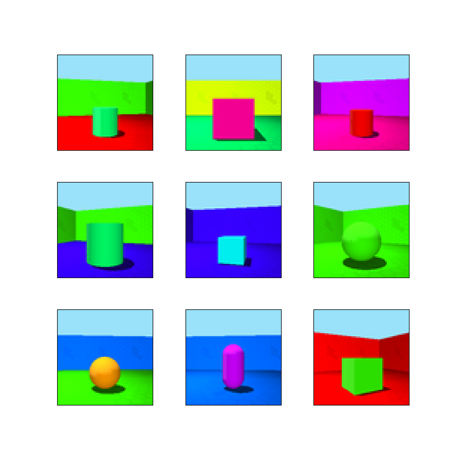
Each image is a huge vector of pixels \({\textcolor{input}{\boldsymbol{x}}}\in \mathbb{R}^{H \times W \times C}\), where \(H\) is the height, \(W\) is the width and \(C\) is the number of channels (in this case, \(64 \times 64 \times 3\)).

Each image can be described by a set of 6 latent variables: floor, wall and object color, shape, orientation and scale.

Latent variable models

Latent variables are unobserved variables, we cannot measure them directly, but we can infer them from the observed data.

In math terms, we model our data distribution as a marginal of the joint distribution of the observed data and the latent variables:

\[ p({\textcolor{input}{\boldsymbol{x}}}) = \int p({\textcolor{input}{\boldsymbol{x}}}, {\textcolor{latent}{\boldsymbol{z}}}) \dd{\textcolor{latent}{\boldsymbol{z}}}\quad \text{or} \quad p({\textcolor{input}{\boldsymbol{x}}}) = \sum_{i} p({\textcolor{input}{\boldsymbol{x}}}, {\textcolor{latent}{\boldsymbol{z}}}_i) \]

where \(p({\textcolor{input}{\boldsymbol{x}}}, {\textcolor{latent}{\boldsymbol{z}}})\) is the joint distribution of the observed data and the latent variables.

Mixture models

In mixture models, we assume that the data is generated from a mixture of several distributions

\[ p({\textcolor{input}{\boldsymbol{x}}}) = \sum_i p({\textcolor{input}{\boldsymbol{x}}}, {\textcolor{latent}{\boldsymbol{z}}}_i) = \sum_i p({\textcolor{input}{\boldsymbol{x}}}\mid{\textcolor{latent}{\boldsymbol{z}}}_i)p({\textcolor{latent}{\boldsymbol{z}}}_i) \]

where \(p({\textcolor{latent}{\boldsymbol{z}}})\) is the mixture distribution and \(p({\textcolor{input}{\boldsymbol{x}}}\mid{\textcolor{latent}{\boldsymbol{z}}})\) is the conditional distribution of the data given the latent variables.

The latent variables \({\textcolor{latent}{\boldsymbol{z}}}\) are often called clusters.
The likelihood is often assumed to be Gaussian, i.e., \(p({\textcolor{input}{\boldsymbol{x}}}\mid{\textcolor{latent}{\boldsymbol{z}}}) = \mathcal{N}({\textcolor{input}{\boldsymbol{x}}}\mid\boldsymbol{\mu}_k, \boldsymbol{\Sigma}_k)\).
The prior is often assumed to be a categorical distribution, i.e., \(p({\textcolor{latent}{\boldsymbol{z}}}) = \text{Cat}({\textcolor{latent}{\boldsymbol{z}}}\mid\boldsymbol{\pi})\).

Gaussian Mixture Models

Modeling the data distribution

1-hot encoding of the discrete latent variable \(\textcolor{latent}{z}_k \in \{0,1\}\), with prior: \[ p(\textcolor{latent}{z}_k=1) = \pi_k \quad \text{and} \quad \sum_k \pi_k = 1 \]
The conditional distribution of the data given the latent variable is: \[ p({\textcolor{input}{\boldsymbol{x}}}\mid\textcolor{latent}{z}_k=1) = {\mathcal{N}}({\textcolor{input}{\boldsymbol{x}}}; {\boldsymbol{\mu}}_k, {\boldsymbol{\Sigma}}_k) \]
The joint distribution of the data and the latent variable is: \[ p({\textcolor{input}{\boldsymbol{x}}}, \textcolor{latent}{z}_k=1) = p({\textcolor{input}{\boldsymbol{x}}}\mid\textcolor{latent}{z}_k=1)p(\textcolor{latent}{z}_k=1) = \pi_k{\mathcal{N}}({\textcolor{input}{\boldsymbol{x}}}; {\boldsymbol{\mu}}_k, {\boldsymbol{\Sigma}}_k) \]
The marginal distribution of the data is: \[ p({\textcolor{input}{\boldsymbol{x}}}) = \sum_k p({\textcolor{input}{\boldsymbol{x}}}, \textcolor{latent}{z}_k=1) = \sum_k \pi_k{\mathcal{N}}({\textcolor{input}{\boldsymbol{x}}}; {\boldsymbol{\mu}}_k, {\boldsymbol{\Sigma}}_k) \]

Posterior distribution

We are interested in the posterior distribution of a cluster assignment given the data:

\[ \begin{aligned} p(\textcolor{latent}{z}_k=1\mid{\textcolor{input}{\boldsymbol{x}}}) &= \frac{p({\textcolor{input}{\boldsymbol{x}}}\mid\textcolor{latent}{z}_k=1)p(\textcolor{latent}{z}_k=1)}{p({\textcolor{input}{\boldsymbol{x}}})} \\ &= \frac{p({\textcolor{input}{\boldsymbol{x}}}\mid\textcolor{latent}{z}_k=1)p(\textcolor{latent}{z}_k=1)}{\sum_{j} p({\textcolor{input}{\boldsymbol{x}}}\mid\textcolor{latent}{z}_j=1)p(\textcolor{latent}{z}_j=1)} \\ &= \frac{\pi_k{\mathcal{N}}({\textcolor{input}{\boldsymbol{x}}}; {\boldsymbol{\mu}}_k, {\boldsymbol{\Sigma}}_k)}{\sum_{j} \pi_j{\mathcal{N}}({\textcolor{input}{\boldsymbol{x}}}; {\boldsymbol{\mu}}_j, {\boldsymbol{\Sigma}}_j)} := \gamma(\textcolor{latent}{z}_k) \end{aligned} \]

\(\gamma(\textcolor{latent}{z}_k)\) is the responsibility of cluster \(k\) for data point \({\textcolor{input}{\boldsymbol{x}}}\).

Log-likelihood

Given a dataset \({\textcolor{input}{\boldsymbol{X}}}= \{{\textcolor{input}{\boldsymbol{x}}}_1, \ldots, {\textcolor{input}{\boldsymbol{x}}}_N\}\) i.i.d, the log-likelihood of the data is:

\[ \begin{aligned} \log p({\textcolor{input}{\boldsymbol{X}}}\mid {\boldsymbol{\pi}}, \{{\boldsymbol{\mu}}_k\}, \{{\boldsymbol{\Sigma}}_k\}) &= \log \prod_{i=1}^N p({\textcolor{input}{\boldsymbol{x}}}_i) \\ &= \sum_{i=1}^N \log p({\textcolor{input}{\boldsymbol{x}}}_i\mid {\boldsymbol{\pi}}, \{{\boldsymbol{\mu}}_k\}, \{{\boldsymbol{\Sigma}}_k\}) \\ &= \sum_{i=1}^N \log \sum_{k=1}^K p({\textcolor{input}{\boldsymbol{x}}}_i\mid\textcolor{latent}{z}_k=1)p(\textcolor{latent}{z}_k=1) \\ &= \sum_{i=1}^N \log \sum_{k=1}^K \pi_k{\mathcal{N}}({\textcolor{input}{\boldsymbol{x}}}_i; {\boldsymbol{\mu}}_k, {\boldsymbol{\Sigma}}_k) \\ \end{aligned} \]

Warning

We cannot simplify it further, because the log and the sum do not commute. How can we optimize it?

Expectation-Maximization algorithm

We need to maximize the log-likelihood of the data w.r.t. the parameters \({\boldsymbol{\pi}}\), \(\{{\boldsymbol{\mu}}_k\}\) and \(\{{\boldsymbol{\Sigma}}_k\}\), for \(k=1,\ldots,K\)

\[ \log p({\textcolor{input}{\boldsymbol{X}}}) = \sum_{i=1}^N \log \sum_{k=1}^K \pi_k{\mathcal{N}}({\textcolor{input}{\boldsymbol{x}}}_i; {\boldsymbol{\mu}}_k, {\boldsymbol{\Sigma}}_k) \]

The problem is not convex.
No closed-form solution! Stationary points depend on the posterior \(\gamma(\textcolor{latent}{z}_{nk})\) for each data point \({\textcolor{input}{\boldsymbol{x}}}_n\).
… but we will see that we can write \(\pi_k\), \({\boldsymbol{\mu}}_k\) and \({\boldsymbol{\Sigma}}_k\) in terms of \(\gamma(\textcolor{latent}{z}_{nk})\).
We can find the local minima by iterative algorithm: alternate update of the expected posterior \(\gamma(\textcolor{latent}{z}_{nk})\) and the maximized parameters \(\pi_k\), \({\boldsymbol{\mu}}_k\) and \({\boldsymbol{\Sigma}}_k\).

Expectation-Maximization algorithm

E-step: compute the expected posterior \(\gamma(\textcolor{latent}{z}_{nk})\) given the current parameters \({\boldsymbol{\pi}}\), \(\{{\boldsymbol{\mu}}_k\}\) and \(\{{\boldsymbol{\Sigma}}_k\}\): \[ \gamma(\textcolor{latent}{z}_{nk}) = \frac{{\mathcal{N}}({\textcolor{input}{\boldsymbol{x}}}_n; {\boldsymbol{\mu}}_k, {\boldsymbol{\Sigma}}_k)\pi_k}{\sum_{j=1}^K {\mathcal{N}}({\textcolor{input}{\boldsymbol{x}}}_n; {\boldsymbol{\mu}}_j, {\boldsymbol{\Sigma}}_j)\pi_j} \]
M-step: update the parameters \({\boldsymbol{\pi}}\), \(\{{\boldsymbol{\mu}}_k\}\) and \(\{{\boldsymbol{\Sigma}}_k\}\) to maximize the expected log-likelihood, given the current expected posterior \(\gamma(\textcolor{latent}{z}_{nk})\). This can be solved in closed form: \[ \begin{aligned} N_k &= \sum_{n=1}^N \gamma(\textcolor{latent}{z}_{nk}) \qquad \pi_k = \frac{N_k}{N} \\ {\boldsymbol{\mu}}_k &= \frac{1}{N_k}\sum_{n=1}^N \gamma(\textcolor{latent}{z}_{nk}){\textcolor{input}{\boldsymbol{x}}}_n \\ {\boldsymbol{\Sigma}}_k &= \frac{1}{N_k}\sum_{n=1}^N \gamma(\textcolor{latent}{z}_{nk})({\textcolor{input}{\boldsymbol{x}}}_n - {\boldsymbol{\mu}}_k)({\textcolor{input}{\boldsymbol{x}}}_n - {\boldsymbol{\mu}}_k)^\top \end{aligned} \]

Example

Derivation of the M-step updates

Results of results for Gaussian distributions

Assume \(p({\textcolor{input}{\boldsymbol{x}}}) = {\mathcal{N}}({\textcolor{input}{\boldsymbol{x}}}; {\boldsymbol{\mu}}, {\boldsymbol{\Sigma}}) = (2\pi)^{-\frac{d}{2}}\det({\boldsymbol{\Sigma}})^{-\frac{1}{2}}\exp\left(-\frac{1}{2}({\textcolor{input}{\boldsymbol{x}}}- {\boldsymbol{\mu}})^\top{\boldsymbol{\Sigma}}^{-1}({\textcolor{input}{\boldsymbol{x}}}- {\boldsymbol{\mu}})\right)\).

Then,

\[ \frac{\partial p({\textcolor{input}{\boldsymbol{x}}})}{\partial {\boldsymbol{\mu}}} = {\mathcal{N}}({\textcolor{input}{\boldsymbol{x}}}; {\boldsymbol{\mu}}, {\boldsymbol{\Sigma}})({\textcolor{input}{\boldsymbol{x}}}- {\boldsymbol{\mu}}){\boldsymbol{\Sigma}}^{-1} \]

and

\[ \frac{\partial p({\textcolor{input}{\boldsymbol{x}}})}{\partial {\boldsymbol{\Sigma}}} = -\frac{1}{2}{\mathcal{N}}({\textcolor{input}{\boldsymbol{x}}}; {\boldsymbol{\mu}}, {\boldsymbol{\Sigma}})\left({\boldsymbol{\Sigma}}^{-1} - {\boldsymbol{\Sigma}}^{-1}({\textcolor{input}{\boldsymbol{x}}}- {\boldsymbol{\mu}})({\textcolor{input}{\boldsymbol{x}}}- {\boldsymbol{\mu}})^\top{\boldsymbol{\Sigma}}^{-1} \right) \]

Derivation of the M-step updates (\({\boldsymbol{\mu}}_k\))

\[ \begin{aligned} \arg\max_{{\boldsymbol{\mu}}_k} p({\textcolor{input}{\boldsymbol{X}}}\mid {\boldsymbol{\pi}}, \{{\boldsymbol{\mu}}_j\}, \{{\boldsymbol{\Sigma}}_j\}) &= \arg\max_{{\boldsymbol{\mu}}_k} \sum_{n=1}^N \log p({\textcolor{input}{\boldsymbol{x}}}_n\mid {\boldsymbol{\pi}}, \{{\boldsymbol{\mu}}_j\}, \{{\boldsymbol{\Sigma}}_j\}) \end{aligned} \]

Compute the partial derivative w.r.t. \({\boldsymbol{\mu}}_k\):

\[ \begin{aligned} \frac{\partial}{\partial {\boldsymbol{\mu}}_k} \log p({\textcolor{input}{\boldsymbol{X}}}\mid {\boldsymbol{\pi}}, \{{\boldsymbol{\mu}}_k\}, \{{\boldsymbol{\Sigma}}_k\}) &= \sum_{n=1}^N \frac{1}{p({\textcolor{input}{\boldsymbol{x}}}_n\mid {\boldsymbol{\pi}}, \{{\boldsymbol{\mu}}_k\}, \{{\boldsymbol{\Sigma}}_k\})}\frac{\partial p({\textcolor{input}{\boldsymbol{x}}}_n\mid {\boldsymbol{\pi}}, \{{\boldsymbol{\mu}}_j\}, \{{\boldsymbol{\Sigma}}_j\})}{\partial {\boldsymbol{\mu}}_k} \\ &= \sum_{n=1}^N \frac{1}{p({\textcolor{input}{\boldsymbol{x}}}_n\mid {\boldsymbol{\pi}}, \{{\boldsymbol{\mu}}_k\}, \{{\boldsymbol{\Sigma}}_k\})}\frac{\partial \pi_k{\mathcal{N}}({\textcolor{input}{\boldsymbol{x}}}_n; {\boldsymbol{\mu}}_k, {\boldsymbol{\Sigma}}_k)}{\partial {\boldsymbol{\mu}}_k} \\ &= \sum_{n=1}^N \frac{\pi_k{\mathcal{N}}({\textcolor{input}{\boldsymbol{x}}}_n; {\boldsymbol{\mu}}_k, {\boldsymbol{\Sigma}}_k)}{\sum_{j=1}^K \pi_j{\mathcal{N}}({\textcolor{input}{\boldsymbol{x}}}_n; {\boldsymbol{\mu}}_j, {\boldsymbol{\Sigma}}_j)}({\textcolor{input}{\boldsymbol{x}}}_n - {\boldsymbol{\mu}}_k){\boldsymbol{\Sigma}}_k^{-1} \\ &= \sum_{n=1}^N \gamma(\textcolor{latent}{z}_{nk})({\textcolor{input}{\boldsymbol{x}}}_n - {\boldsymbol{\mu}}_k){\boldsymbol{\Sigma}}_k^{-1} = 0 \quad \Rightarrow {\boldsymbol{\mu}}_k = \frac{\sum_{n=1}^N \gamma(\textcolor{latent}{z}_{nk}){\textcolor{input}{\boldsymbol{x}}}_n}{\sum_{n=1}^N \gamma(\textcolor{latent}{z}_{nk})} \end{aligned} \]

Derivation of the M-step updates (\({\boldsymbol{\Sigma}}_k\), \({\boldsymbol{\pi}}\))

Same for the covariance:

Write the derivative of the log-likelihood w.r.t. \({\boldsymbol{\Sigma}}_k\) (use the properties of the Gaussian distribution).
Manipulate it to make \(\gamma(\textcolor{latent}{z}_{nk})\) appear.
Set it to zero and solve for \({\boldsymbol{\Sigma}}_k\).

Same for the weights \({\boldsymbol{\pi}}\), but we have to use the constraint \(\sum_{k=1}^K \pi_k = 1\).

Use Lagrange multipliers to introduce a new variable \(\lambda\) and write the Lagrangian function: \[ \ell({\boldsymbol{\pi}}, \lambda) = \log p({\textcolor{input}{\boldsymbol{X}}}\mid {\boldsymbol{\pi}}, \{{\boldsymbol{\mu}}_k\}, \{{\boldsymbol{\Sigma}}_k\}) + \lambda\left(1 - \sum_{k=1}^K \pi_k\right) \]
Compute the partial derivative w.r.t. \({\boldsymbol{\pi}}\) and \(\lambda\)
Set them to zero and solve for \({\boldsymbol{\pi}}\) and \(\lambda\).

EM for Gaussian Mixture Models

Algorithm:

Initialize the parameters \({\boldsymbol{\pi}}\), \(\{{\boldsymbol{\mu}}_k\}\) and \(\{{\boldsymbol{\Sigma}}_k\}\)
Repeat until convergence (likelihood does not change significantly):
1. E-step: compute the expected posterior \(\gamma(\textcolor{latent}{z}_{nk})\) given the current parameters \({\boldsymbol{\pi}}\), \(\{{\boldsymbol{\mu}}_k\}\) and \(\{{\boldsymbol{\Sigma}}_k\}\):
2. M-step: update the parameters \({\boldsymbol{\pi}}\), \(\{{\boldsymbol{\mu}}_k\}\) and \(\{{\boldsymbol{\Sigma}}_k\}\) to maximize the expected log-likelihood, given the current expected posterior \(\gamma(\textcolor{latent}{z}_{nk})\):
3. Compute the log-likelihood of the data given the current parameters \({\boldsymbol{\pi}}\), \(\{{\boldsymbol{\mu}}_k\}\) and \(\{{\boldsymbol{\Sigma}}_k\}\)

Important:

EM is guaranteed to converge to a local maximum, not necessarily to the global maximum.
EM is sensitive to the initialization of the parameters (try different initializations and choose the one that gives the highest log-likelihood)

Gaussian Mixture Models

After the EM algorithm converges, we can the learned parameters to:

Generate new data points by sampling from the mixture model.
Compute the likelihood of new data points.
Compute the posterior distribution of the latent variables given new data points (e.g., clustering).

Gaussian Mixture Models

Pros:

Simple and easy to implement.
Can model any distribution as a mixture of Gaussians.
One model can be used for different tasks (e.g., clustering, density estimation, generation).

Cons:

Sensitive to the initialization of the parameters, can get stuck in local minima.
The number of clusters \(K\) must be specified in advance.
The number of clusters \(K\) must be small, otherwise the model will overfit the data.

Question: Can we be Bayesian about the number of clusters \(K\)? Yes, it’s called Dirichlet Process Mixture Model (DPMM)

Dimensionality reduction as a generative model

Linear latent variable models

Linear latent variable models are a class of generative models that assume that the data is generated from a linear combination of latent variables.

We will:

Review the Principal Component Analysis (PCA) algorithm.
Introduce the (probabilistic) PCA as a linear latent variable model.

Principal Component Analysis

Assume we have a dataset \({\textcolor{input}{\boldsymbol{X}}}= \{{\textcolor{input}{\boldsymbol{x}}}_1, \ldots, {\textcolor{input}{\boldsymbol{x}}}_N\}\), where \({\textcolor{input}{\boldsymbol{x}}}_n\in{\mathbb{R}}^{D}\).
We want to find a low-dimensional representation of the data, i.e., we want to find a mapping \({\textcolor{input}{\boldsymbol{x}}}_n \mapsto {\textcolor{latent}{\boldsymbol{z}}}_n\) such that \({\textcolor{latent}{\boldsymbol{z}}}_n\in{\mathbb{R}}^{K}\), where \(K < D\).
Choose the mapping such that the variance of the data is maximized, i.e., we want to find the mapping that maximizes the variance of the data in the low-dimensional space.

Principal Component Analysis

We want to find the direction of maximum variance, i.e., the direction that maximizes the variance of the data in the low-dimensional space.

How to find the direction of maximum variance?

Let’s start by projecting the data on 1D subspace \(\textcolor{latent}{z}= {\textcolor{params}{\boldsymbol{w}}}^\top{\textcolor{input}{\boldsymbol{x}}}\), where \({\textcolor{params}{\boldsymbol{w}}}\in{\mathbb{R}}^{D}\).
We only want the direction, so we can assume that \(\norm{{\textcolor{params}{\boldsymbol{w}}}} = 1\).
Given data \({\textcolor{input}{\boldsymbol{X}}}= \{{\textcolor{input}{\boldsymbol{x}}}_1, \ldots, {\textcolor{input}{\boldsymbol{x}}}_N\}\), we maximize the variance of the projected data \({\textcolor{latent}{\boldsymbol{z}}}= {\textcolor{input}{\boldsymbol{X}}}{\textcolor{params}{\boldsymbol{w}}}\) constrained to \(\norm{{\textcolor{params}{\boldsymbol{w}}}} = 1\): \[ \arg\max_{{\textcolor{params}{\boldsymbol{w}}}} \norm{{\textcolor{latent}{\boldsymbol{z}}}}^2 \qquad \text{s.t.} \quad \norm{{\textcolor{params}{\boldsymbol{w}}}}^2 = 1 \]

Assumes that \({\textcolor{input}{\boldsymbol{X}}}\) is centered (i.e., \({\textcolor{input}{\boldsymbol{X}}}\) has zero mean)

Analytic solution

Let’s use the Lagrange multipliers to solve the constrained optimization problem:

\[ \ell({\textcolor{params}{\boldsymbol{w}}}, \lambda) = \norm{{\textcolor{latent}{\boldsymbol{z}}}}^2 - \lambda(\norm{{\textcolor{params}{\boldsymbol{w}}}}^2 - 1) = {\textcolor{params}{\boldsymbol{w}}}^\top{\textcolor{input}{\boldsymbol{X}}}^\top{\textcolor{input}{\boldsymbol{X}}}{\textcolor{params}{\boldsymbol{w}}}- \lambda({\textcolor{params}{\boldsymbol{w}}}^\top{\textcolor{params}{\boldsymbol{w}}}- 1) \]

Compute the partial derivative w.r.t. \({\textcolor{params}{\boldsymbol{w}}}\) and \(\lambda\):

\[ \begin{aligned} \frac{\partial \ell}{\partial {\textcolor{params}{\boldsymbol{w}}}} &= 2{\textcolor{input}{\boldsymbol{X}}}^\top{\textcolor{input}{\boldsymbol{X}}}{\textcolor{params}{\boldsymbol{w}}}- 2\lambda{\textcolor{params}{\boldsymbol{w}}}= 0 \quad \Rightarrow \quad {\textcolor{input}{\boldsymbol{X}}}^\top{\textcolor{input}{\boldsymbol{X}}}{\textcolor{params}{\boldsymbol{w}}}= \lambda{\textcolor{params}{\boldsymbol{w}}}\\ \frac{\partial \ell}{\partial \lambda} &= -({\textcolor{params}{\boldsymbol{w}}}^\top{\textcolor{params}{\boldsymbol{w}}}- 1) = 0 \end{aligned} \]

This is an eigenvalue problem, where \(\lambda\) is the eigenvalue and \({\textcolor{params}{\boldsymbol{w}}}\) is the eigenvector of the covariance matrix \({\textcolor{input}{\boldsymbol{X}}}^\top{\textcolor{input}{\boldsymbol{X}}}\).

Analytic solution

But which eigenvalue?

The eigenvalue \(\lambda\) is the variance of the projected data \({\textcolor{latent}{\boldsymbol{z}}}\): \(\lambda = {\textcolor{params}{\boldsymbol{w}}}^\top{\textcolor{input}{\boldsymbol{X}}}^\top{\textcolor{input}{\boldsymbol{X}}}{\textcolor{params}{\boldsymbol{w}}}\)
If we want to maximize the variance, we need to find the largest eigenvalue of the covariance matrix \({\textcolor{input}{\boldsymbol{X}}}^\top{\textcolor{input}{\boldsymbol{X}}}\).
The corresponding eigenvector is the direction of maximum variance: \(\widehat{\textcolor{params}{\boldsymbol{w}}}\)

Probabilistic PCA

PCA can be seen as a linear continuous latent variable model, where the latent variable \({\textcolor{latent}{\boldsymbol{z}}}\) is a linear combination of the observed data \({\textcolor{input}{\boldsymbol{x}}}\).
Question: Can we approach PCA from a probabilistic point of view? Answer: Yes!

Recall the continuous latent variable model:

\[ p({\textcolor{input}{\boldsymbol{x}}}) = \int p({\textcolor{input}{\boldsymbol{x}}}, {\textcolor{latent}{\boldsymbol{z}}}) \dd{\textcolor{latent}{\boldsymbol{z}}}= \int p({\textcolor{input}{\boldsymbol{x}}}\mid{\textcolor{latent}{\boldsymbol{z}}})p({\textcolor{latent}{\boldsymbol{z}}}) \dd{\textcolor{latent}{\boldsymbol{z}}} \]

PPCA Modeling Assumptions

The generative model works as follows:

\[ {\textcolor{input}{\boldsymbol{x}}}= {\textcolor{params}{\boldsymbol{W}}}{\textcolor{latent}{\boldsymbol{z}}}+ {\boldsymbol{\mu}}+ {\textcolor{noise}{\boldsymbol{\varepsilon}}} \]

where:

\({\textcolor{params}{\boldsymbol{W}}}\in{\mathbb{R}}^{D\times K}\) is the weight matrix
\({\textcolor{latent}{\boldsymbol{z}}}\in{\mathbb{R}}^{K}\) is the latent variable
\({\boldsymbol{\mu}}\in{\mathbb{R}}^{D}\) is the mean of the data
\({\textcolor{noise}{\boldsymbol{\varepsilon}}}\in{\mathbb{R}}^{D}\) is the noise

How can we treat these variables?

PPCA Modeling Assumptions

The latent variable \({\textcolor{latent}{\boldsymbol{z}}}\) is assumed to be a standard Gaussian distribution: \[ p({\textcolor{latent}{\boldsymbol{z}}}) = {\mathcal{N}}({\textcolor{latent}{\boldsymbol{z}}}; 0, {\boldsymbol{I}}) \]
The noise \({\textcolor{noise}{\boldsymbol{\varepsilon}}}\) is assumed to be a Gaussian distribution with zero mean and covariance matrix \(\sigma^2{\boldsymbol{I}}\): \[ p({\textcolor{noise}{\boldsymbol{\varepsilon}}}) = {\mathcal{N}}({\textcolor{noise}{\boldsymbol{\varepsilon}}}; 0, \sigma^2{\boldsymbol{I}}) \]

The observed data \({\textcolor{input}{\boldsymbol{x}}}\) conditioned on the latent variable \({\textcolor{latent}{\boldsymbol{z}}}\) is a Gaussian distribution \[ p({\textcolor{input}{\boldsymbol{x}}}\mid {\textcolor{latent}{\boldsymbol{z}}}) = {\mathcal{N}}({\textcolor{input}{\boldsymbol{x}}}; {\textcolor{params}{\boldsymbol{W}}}{\textcolor{latent}{\boldsymbol{z}}}+ {\boldsymbol{\mu}}, \sigma^2{\boldsymbol{I}}) \]
The marginal distribution of the data \({\textcolor{input}{\boldsymbol{x}}}\) is obtained by integrating out the latent variable \({\textcolor{latent}{\boldsymbol{z}}}\):

\[ p({\textcolor{input}{\boldsymbol{x}}}) = \int p({\textcolor{input}{\boldsymbol{x}}}\mid{\textcolor{latent}{\boldsymbol{z}}})p({\textcolor{latent}{\boldsymbol{z}}}) \dd{\textcolor{latent}{\boldsymbol{z}}}= \int {\mathcal{N}}({\textcolor{input}{\boldsymbol{x}}}; {\textcolor{params}{\boldsymbol{W}}}{\textcolor{latent}{\boldsymbol{z}}}+ {\boldsymbol{\mu}}, \sigma^2{\boldsymbol{I}}){\mathcal{N}}({\textcolor{latent}{\boldsymbol{z}}}; 0, {\boldsymbol{I}}) \dd{\textcolor{latent}{\boldsymbol{z}}} \]

It’s a Gaussian distribution \({\mathcal{N}}(?, ?)\).

PPCA Modeling Assumptions

For the mean, we have:

\[ \begin{aligned} \mathbb{E}{[{\textcolor{input}{\boldsymbol{x}}}]} &= \mathbb{E}{[{\textcolor{params}{\boldsymbol{W}}}{\textcolor{latent}{\boldsymbol{z}}}+ {\boldsymbol{\mu}}+ {\textcolor{noise}{\boldsymbol{\varepsilon}}}]} \\ &= {\textcolor{params}{\boldsymbol{W}}}\mathbb{E}{[{\textcolor{latent}{\boldsymbol{z}}}]} + {\boldsymbol{\mu}}+ \mathbb{E}{[{\textcolor{noise}{\boldsymbol{\varepsilon}}}]} \\ &= {\textcolor{params}{\boldsymbol{W}}}\cdot 0 + {\boldsymbol{\mu}}+ 0 = {\boldsymbol{\mu}} \end{aligned} \]

For the covariance, we have:

\[ \begin{aligned} \text{Cov}({\textcolor{input}{\boldsymbol{x}}}) &= \mathbb{E}[({\textcolor{input}{\boldsymbol{x}}}- {\boldsymbol{\mu}})({\textcolor{input}{\boldsymbol{x}}}- {\boldsymbol{\mu}})^\top] \\ &= \mathbb{E}[({\textcolor{params}{\boldsymbol{W}}}{\textcolor{latent}{\boldsymbol{z}}}+ {\textcolor{noise}{\boldsymbol{\varepsilon}}})({\textcolor{params}{\boldsymbol{W}}}{\textcolor{latent}{\boldsymbol{z}}}+ {\textcolor{noise}{\boldsymbol{\varepsilon}}})^\top] \\ &= \mathbb{E}[{\textcolor{params}{\boldsymbol{W}}}{\textcolor{latent}{\boldsymbol{z}}}{\textcolor{latent}{\boldsymbol{z}}}^\top{\textcolor{params}{\boldsymbol{W}}}^\top + {\textcolor{noise}{\boldsymbol{\varepsilon}}}{\textcolor{noise}{\boldsymbol{\varepsilon}}}^\top + {\textcolor{params}{\boldsymbol{W}}}{\textcolor{latent}{\boldsymbol{z}}}{\textcolor{noise}{\boldsymbol{\varepsilon}}}^\top + {\textcolor{noise}{\boldsymbol{\varepsilon}}}{\textcolor{latent}{\boldsymbol{z}}}^\top{\textcolor{params}{\boldsymbol{W}}}] \\ &= {\textcolor{params}{\boldsymbol{W}}}\mathbb{E}[{\textcolor{latent}{\boldsymbol{z}}}{\textcolor{latent}{\boldsymbol{z}}}^\top]{\textcolor{params}{\boldsymbol{W}}}^\top + \mathbb{E}[{\textcolor{noise}{\boldsymbol{\varepsilon}}}{\textcolor{noise}{\boldsymbol{\varepsilon}}}^\top] + {\textcolor{params}{\boldsymbol{W}}}\mathbb{E}[{\textcolor{latent}{\boldsymbol{z}}}]\mathbb{E}[{\textcolor{noise}{\boldsymbol{\varepsilon}}}^\top] + \mathbb{E}[{\textcolor{noise}{\boldsymbol{\varepsilon}}}]\mathbb{E}[{\textcolor{latent}{\boldsymbol{z}}}^\top]{\textcolor{params}{\boldsymbol{W}}}\\ &= {\textcolor{params}{\boldsymbol{W}}}\cdot {\boldsymbol{I}}\cdot{\textcolor{params}{\boldsymbol{W}}}^\top + \sigma^2{\boldsymbol{I}}+ 0 + 0 \\ &= {\textcolor{params}{\boldsymbol{W}}}{\textcolor{params}{\boldsymbol{W}}}^\top + \sigma^2{\boldsymbol{I}} \end{aligned} \]

PPCA in a picture

PPCA Solution

Now, we need to find the parameters \({\textcolor{params}{\boldsymbol{W}}}\), \({\boldsymbol{\mu}}\) and \(\sigma^2\) that maximize the log-likelihood of the data: \[ \begin{aligned} \log p({\textcolor{input}{\boldsymbol{X}}}; {\textcolor{params}{\boldsymbol{W}}}, {\boldsymbol{\mu}}, \sigma^2) &= \sum_{n=1}^N \log p({\textcolor{input}{\boldsymbol{x}}}_n; {\textcolor{params}{\boldsymbol{W}}}, {\boldsymbol{\mu}}, \sigma^2) = \sum_{n=1}^N \log {\mathcal{N}}({\textcolor{input}{\boldsymbol{x}}}_n; {\boldsymbol{\mu}}, {\textcolor{params}{\boldsymbol{W}}}{\textcolor{params}{\boldsymbol{W}}}^\top + \sigma^2{\boldsymbol{I}})\\ &= -\frac{NK}{2}\log(2\pi) - \frac{N}{2}\log(\det({\textcolor{params}{\boldsymbol{W}}}{\textcolor{params}{\boldsymbol{W}}}^\top + \sigma^2{\boldsymbol{I}})) - \frac{1}{2}\sum_{n=1}^N ({\textcolor{input}{\boldsymbol{x}}}_n - {\boldsymbol{\mu}})^\top({\textcolor{params}{\boldsymbol{W}}}{\textcolor{params}{\boldsymbol{W}}}^\top + \sigma^2{\boldsymbol{I}})^{-1}({\textcolor{input}{\boldsymbol{x}}}_n - {\boldsymbol{\mu}}) \end{aligned} \]

Again, compute the partial derivative w.r.t. \({\textcolor{params}{\boldsymbol{W}}}\), \({\boldsymbol{\mu}}\) and \(\sigma^2\) and set them to zero.

PPCA Solution

Let’s define the sample covariance matrix \({\boldsymbol{S}}= {\textcolor{input}{\boldsymbol{X}}}{\textcolor{input}{\boldsymbol{X}}}^\top\). Solutions for \({\textcolor{params}{\boldsymbol{W}}}\), \({\boldsymbol{\mu}}\) and \(\sigma^2\) can be found in closed form, no need to use the EM algorithm.

For the mean, we have: \({\boldsymbol{\mu}}= \frac{1}{N}\sum_{n=1}^N {\textcolor{input}{\boldsymbol{x}}}_n\)

For the noise variance, we have: \(\sigma^2 = \frac{1}{D-K} \sum_{j=K+1}^D \lambda_j\), where \(\lambda_j\) are the eigenvalues of \({\boldsymbol{S}}\)

For the weight matrix, we have: \({\textcolor{params}{\boldsymbol{W}}}= {\boldsymbol{U}}_K({\boldsymbol{\Lambda}}_K - \sigma^2{\boldsymbol{I}})^{1/2}\), where \({\boldsymbol{U}}_K\) are the first \(K\) eigenvectors \({\boldsymbol{S}}\) and \({\boldsymbol{\Lambda}}_K\) is the diagonal matrix of the first \(K\) eigenvalues.

Because everything is Gaussian, we can also compute the posterior distribution of the latent variable \({\textcolor{latent}{\boldsymbol{z}}}\) given the data \({\textcolor{input}{\boldsymbol{x}}}\):

\[ p({\textcolor{latent}{\boldsymbol{z}}}_n\mid{\textcolor{input}{\boldsymbol{x}}}_n) = {\mathcal{N}}({\textcolor{latent}{\boldsymbol{z}}}_n; {\boldsymbol{C}}^{-1}{\textcolor{params}{\boldsymbol{W}}}^\top({\textcolor{input}{\boldsymbol{x}}}_n - {\boldsymbol{\mu}}), \sigma^2{\boldsymbol{C}}^{-1}) \]

with \({\boldsymbol{C}}= {\textcolor{params}{\boldsymbol{W}}}^\top{\textcolor{params}{\boldsymbol{W}}}+ \sigma^2{\boldsymbol{I}}\)

Is the PPCA solution the same as PCA?

The PPCA solution is more general than PCA, because it assumes that the data is generated from a Gaussian distribution with noise.

PPCA Recipe

Start from a model for the data \({\textcolor{input}{\boldsymbol{x}}}\) given the latent variable \({\textcolor{latent}{\boldsymbol{z}}}\) and the linear weight \({\textcolor{params}{\boldsymbol{W}}}\):

Place a prior on the latent variable \(p({\textcolor{latent}{\boldsymbol{z}}})\)
Marginalize the latent variable \({\textcolor{latent}{\boldsymbol{z}}}\) to obtain the marginal distribution of the data p(\({\textcolor{input}{\boldsymbol{x}}}\); \({\textcolor{params}{\boldsymbol{W}}}\))
Maximize the log-likelihood of the data w.r.t. the parameters \({\textcolor{params}{\boldsymbol{W}}}\)

But we could have also done the following:

We place a prior the linear weight \(p({\textcolor{params}{\boldsymbol{W}}})\).
We marginalize linear weight \({\textcolor{params}{\boldsymbol{W}}}\) to obtain the marginal distribution of the data p(\({\textcolor{input}{\boldsymbol{x}}}\); \({\textcolor{latent}{\boldsymbol{z}}}\))
We maximize the log-likelihood of the data w.r.t. the \({\textcolor{latent}{\boldsymbol{z}}}\)

This is a step closer to probabilistic kernel PCA and to the Gaussian process latent variable model (GPLVM).