Review of Approximate Inference
\[
\require{physics}
\definecolor{input}{rgb}{0.42, 0.55, 0.74}
\definecolor{params}{rgb}{0.51,0.70,0.40}
\definecolor{output}{rgb}{0.843, 0.608, 0}
\definecolor{vparams}{rgb}{0.58, 0, 0.83}
\definecolor{noise}{rgb}{0.0, 0.48, 0.65}
\definecolor{latent}{rgb}{0.8, 0.0, 0.8}
\]
\[
\require{physics}
\definecolor{input}{rgb}{0.42, 0.55, 0.74}
\definecolor{params}{rgb}{0.51,0.70,0.40}
\definecolor{output}{rgb}{0.843, 0.608, 0}
\definecolor{vparams}{rgb}{0.58, 0, 0.83}
\definecolor{noise}{rgb}{0.0, 0.48, 0.65}
\]
Where are we?
Given a likelihood \(p({\textcolor{output}{\boldsymbol{y}}}\mid {\textcolor{params}{\boldsymbol{\theta}}})\) and a prior \(p({\textcolor{params}{\boldsymbol{\theta}}})\), the goal is to compute the posterior distribution \(p({\textcolor{params}{\boldsymbol{\theta}}}\mid {\textcolor{output}{\boldsymbol{y}}})\)
\[
p({\textcolor{params}{\boldsymbol{\theta}}}\mid {\textcolor{output}{\boldsymbol{y}}}) = \frac{p({\textcolor{output}{\boldsymbol{y}}}\mid {\textcolor{params}{\boldsymbol{\theta}}}) p({\textcolor{params}{\boldsymbol{\theta}}})}{p({\textcolor{output}{\boldsymbol{y}}})}
\]
We have seen that exact inference is possible if the prior and likelihood are conjugate distributions (e.g. for Bayesian linear regression with Gaussian likelihood and Gaussian prior).
But in most cases, the Bayesian approach is intractable.
- We cannot compute the posterior distribution \(p({\textcolor{params}{\boldsymbol{\theta}}}\mid {\textcolor{output}{\boldsymbol{y}}})\) in closed form.
- We cannot make predictions for a new point \(\textcolor{output}{y}_\star\) in closed form \(p(\textcolor{output}{y}_\star \mid {\textcolor{output}{\boldsymbol{y}}}) = \int p(\textcolor{output}{y}_\star \mid {\textcolor{params}{\boldsymbol{\theta}}}) p({\textcolor{params}{\boldsymbol{\theta}}}\mid {\textcolor{output}{\boldsymbol{y}}}) \dd {\textcolor{params}{\boldsymbol{\theta}}}\).
Last Week
We have seen that we can use Monte Carlo methods to approximate the posterior distribution \(p({\textcolor{params}{\boldsymbol{\theta}}}\mid {\textcolor{output}{\boldsymbol{y}}})\).
- Rejection sampling: sample from a simple distribution and accept/reject samples
- Markov Chain Monte Carlo (MCMC): sample from a Markov chain that converges to the target distribution.
- Metropolis-Hastings: do random walk in the parameter space and accept/reject samples based on the ratio of the target distribution in the current and next state.
- Hamiltonian Monte Carlo (HMC): explore the parameter space by simulating a particle with a potential given by negative log posterior and a random momentum.
This Week
In this week, we will see another way to approximate the posterior distribution \(p({\textcolor{params}{\boldsymbol{\theta}}}\mid {\textcolor{output}{\boldsymbol{y}}})\).
Can we use a simpler distribution to approximate the posterior?
And if so, how?
Laplace Approximation
Idea:
- Let’s find a way to have a local approximation of the posterior distribution \(p({\textcolor{params}{\boldsymbol{\theta}}}\mid {\textcolor{output}{\boldsymbol{y}}})\) around the mode \(\widehat{{\textcolor{params}{\boldsymbol{\theta}}}}\).
![]()
Derivation of Laplace Approximation
Given a likelihood \(p({\textcolor{output}{\boldsymbol{y}}}\mid{\textcolor{params}{\boldsymbol{\theta}}})\) and a prior \(p({\textcolor{params}{\boldsymbol{\theta}}})\), the posterior distribution is given by
\[
p({\textcolor{params}{\boldsymbol{\theta}}}\mid{\textcolor{output}{\boldsymbol{y}}}) = \frac 1 Z \exp\left(-{\mathcal{U}}({\textcolor{params}{\boldsymbol{\theta}}})\right)
\]
where \(Z\) is the normalizing constant and \({\mathcal{U}}({\textcolor{params}{\boldsymbol{\theta}}})= -\log p({\textcolor{output}{\boldsymbol{y}}}\mid{\textcolor{params}{\boldsymbol{\theta}}}) - \log p({\textcolor{params}{\boldsymbol{\theta}}})\) is the (un-normalized) negative log posterior.
Taylor expand \({\mathcal{U}}({\textcolor{params}{\boldsymbol{\theta}}})\) around the mode \(\widehat{{\textcolor{params}{\boldsymbol{\theta}}}}\) to the second order
\[
{\mathcal{U}}({\textcolor{params}{\boldsymbol{\theta}}}) \approx {\mathcal{U}}(\widehat{{\textcolor{params}{\boldsymbol{\theta}}}}) + ({\textcolor{params}{\boldsymbol{\theta}}}-\widehat{{\textcolor{params}{\boldsymbol{\theta}}}})^\top {\boldsymbol{g}}+ \frac 1 2 ({\textcolor{params}{\boldsymbol{\theta}}}-\widehat{{\textcolor{params}{\boldsymbol{\theta}}}})^\top {\boldsymbol{H}}({\textcolor{params}{\boldsymbol{\theta}}}-\widehat{{\textcolor{params}{\boldsymbol{\theta}}}})
\]
where:
- \({\boldsymbol{g}}=\grad{\mathcal{U}}(\widehat{{\textcolor{params}{\boldsymbol{\theta}}}})\) is the gradient
- \({\boldsymbol{H}}=\grad^2{\mathcal{U}}(\widehat{{\textcolor{params}{\boldsymbol{\theta}}}})\) is the Hessian matrix
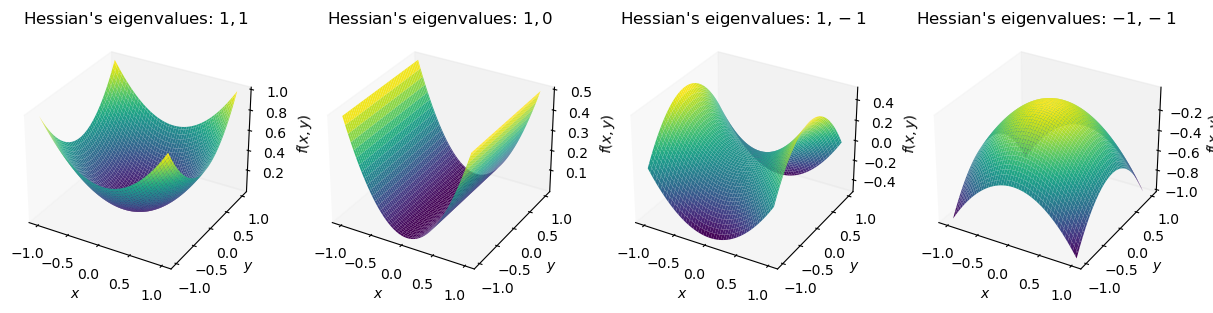
Refresher: Hessians
The Hessian matrix \({\boldsymbol{H}}\) is a square matrix \(D\times D\) of second-order partial derivatives of \({\mathcal{U}}({\textcolor{params}{\boldsymbol{\theta}}})\) computed in \({\textcolor{params}{\boldsymbol{\theta}}}\).
\[
{\boldsymbol{H}}= \grad^2 {\mathcal{U}}({\textcolor{params}{\boldsymbol{\theta}}})\begin{bmatrix}
\frac{\partial^2 {\mathcal{U}}}{\partial {\color{params}\theta}_1^2}({\textcolor{params}{\boldsymbol{\theta}}}) & \frac{\partial^2 {\mathcal{U}}}{\partial {\color{params}\theta}_1\partial {\color{params}\theta}_2}({\textcolor{params}{\boldsymbol{\theta}}}) & \cdots & \frac{\partial^2 {\mathcal{U}}}{\partial {\color{params}\theta}_1\partial {\color{params}\theta}_D}({\textcolor{params}{\boldsymbol{\theta}}}) \\
\frac{\partial^2 {\mathcal{U}}}{\partial {\color{params}\theta}_2\partial {\color{params}\theta}_1}({\textcolor{params}{\boldsymbol{\theta}}}) & \frac{\partial^2 {\mathcal{U}}}{\partial {\color{params}\theta}_2^2}({\textcolor{params}{\boldsymbol{\theta}}}) & \cdots & \frac{\partial^2 {\mathcal{U}}}{\partial {\color{params}\theta}_2\partial {\color{params}\theta}_D}({\textcolor{params}{\boldsymbol{\theta}}}) \\
\cdots & \cdots & \ddots & \cdots \\
\frac{\partial^2 {\mathcal{U}}}{\partial {\color{params}\theta}_D\partial {\color{params}\theta}_1}({\textcolor{params}{\boldsymbol{\theta}}}) & \frac{\partial^2 {\mathcal{U}}}{\partial {\color{params}\theta}_D\partial {\color{params}\theta}_2}({\textcolor{params}{\boldsymbol{\theta}}}) & \cdots & \frac{\partial^2 {\mathcal{U}}}{\partial {\color{params}\theta}_D^2}({\textcolor{params}{\boldsymbol{\theta}}})
\end{bmatrix}
\]
Derivation of Laplace Approximation
\[
{\mathcal{U}}({\textcolor{params}{\boldsymbol{\theta}}}) \approx {\mathcal{U}}(\widehat{{\textcolor{params}{\boldsymbol{\theta}}}}) + ({\textcolor{params}{\boldsymbol{\theta}}}-\widehat{{\textcolor{params}{\boldsymbol{\theta}}}})^\top {\boldsymbol{g}}+ \frac 1 2 ({\textcolor{params}{\boldsymbol{\theta}}}-\widehat{{\textcolor{params}{\boldsymbol{\theta}}}})^\top {\boldsymbol{H}}({\textcolor{params}{\boldsymbol{\theta}}}-\widehat{{\textcolor{params}{\boldsymbol{\theta}}}})
\]
The mode \(\widehat{{\textcolor{params}{\boldsymbol{\theta}}}}\) is the value of \({\textcolor{params}{\boldsymbol{\theta}}}\) that maximizes \(p({\textcolor{params}{\boldsymbol{\theta}}}\mid{\textcolor{output}{\boldsymbol{y}}})\) or equivalently minimizes \({\mathcal{U}}({\textcolor{params}{\boldsymbol{\theta}}})\).
Because we are expanding around the mode, \({\boldsymbol{g}}=\grad{\mathcal{U}}(\widehat{{\textcolor{params}{\boldsymbol{\theta}}}})=0\).
Approximate the posterior distribution with this expansion:
\[
\begin{aligned}
p({\textcolor{params}{\boldsymbol{\theta}}}\mid{\textcolor{output}{\boldsymbol{y}}}) &\approx \frac 1 Z \exp\left(-{\mathcal{U}}(\widehat{{\textcolor{params}{\boldsymbol{\theta}}}}) - \frac 1 2 ({\textcolor{params}{\boldsymbol{\theta}}}-\widehat{{\textcolor{params}{\boldsymbol{\theta}}}})^\top {\boldsymbol{H}}({\textcolor{params}{\boldsymbol{\theta}}}-\widehat{{\textcolor{params}{\boldsymbol{\theta}}}})\right)\\
&= \frac 1 Z \exp\left(-{\mathcal{U}}(\widehat{{\textcolor{params}{\boldsymbol{\theta}}}})\right) \exp\left(-\frac 1 2 ({\textcolor{params}{\boldsymbol{\theta}}}-\widehat{{\textcolor{params}{\boldsymbol{\theta}}}})^\top {\boldsymbol{H}}({\textcolor{params}{\boldsymbol{\theta}}}-\widehat{{\textcolor{params}{\boldsymbol{\theta}}}})\right)
\end{aligned}
\]
Derivation of Laplace Approximation
\[
\begin{aligned}
p({\textcolor{params}{\boldsymbol{\theta}}}\mid{\textcolor{output}{\boldsymbol{y}}}) &\approx \frac 1 Z \exp\left(-{\mathcal{U}}(\widehat{{\textcolor{params}{\boldsymbol{\theta}}}})\right) \exp\left(-\frac 1 2 ({\textcolor{params}{\boldsymbol{\theta}}}-\widehat{{\textcolor{params}{\boldsymbol{\theta}}}})^\top {\boldsymbol{H}}({\textcolor{params}{\boldsymbol{\theta}}}-\widehat{{\textcolor{params}{\boldsymbol{\theta}}}})\right)
\end{aligned}
\]
Compare this to the form of a Gaussian distribution:
\[
\begin{aligned}
{\mathcal{N}}({\textcolor{params}{\boldsymbol{\theta}}}\mid{\boldsymbol{\mu}}, {\boldsymbol{\Sigma}}) &= \frac 1 2 (2\pi)^{D/2}\det({\boldsymbol{\Sigma}})^{-1/2}
\exp\left(-\frac 1 2 ({\textcolor{params}{\boldsymbol{\theta}}}-{\boldsymbol{\mu}})^\top {\boldsymbol{\Sigma}}^{-1}({\textcolor{params}{\boldsymbol{\theta}}}-{\boldsymbol{\mu}})\right)
\end{aligned}
\]
Taylor expansion of the log posterior \(\Rightarrow\) Gaussian approximation of the posterior.
The mean of the Gaussian is the mode of the posterior \(\widehat{{\textcolor{params}{\boldsymbol{\theta}}}}\).
The covariance of the Gaussian is the inverse of the Hessian \({\boldsymbol{H}}^{-1}\).
The normalizing constant is \(Z=(2\pi)^{D/2}\det({\boldsymbol{H}})^{-1/2}\exp(-{\mathcal{U}}(\widehat{{\textcolor{params}{\boldsymbol{\theta}}}}))\).
Practical Considerations
- The mode \(\widehat{{\textcolor{params}{\boldsymbol{\theta}}}}\) can be found by gradient-based optimization
\[
{\textcolor{params}{\boldsymbol{\theta}}}\leftarrow {\textcolor{params}{\boldsymbol{\theta}}}- \eta \grad{\mathcal{U}}({\textcolor{params}{\boldsymbol{\theta}}}) \quad \text{until convergence}
\]
The exact Hessian \({\boldsymbol{H}}\) can be expensive to compute and invert for large \(D\).
- Use a diagonal approximation of the Hessian or a block-diagonal approximation.
The Laplace approximation is only valid in a neighborhood of the mode.
Laplace Approximation: Example
Consider a Gamma distribution with shape parameter \(\alpha\) and rate parameter \(\beta\).
\[
p(x\mid\alpha,\beta) = \frac{\beta^\alpha}{\Gamma(\alpha)} x^{\alpha-1}\exp(-\beta x)
% x^{\alpha-1}\exp(-\beta x)
\]
![]()
Laplace Approximation: Example
Write the negative log posterior \({\mathcal{U}}(x)\). \[
{\mathcal{U}}(x) = -(\alpha-1)\log x + \beta x
\]
Compute the mode \(\widehat{x}\) by setting \(\frac{\dd{\mathcal{U}}(x)}{\dd x}=0\).
\[
\begin{aligned}
\frac{\dd{\mathcal{U}}(x)}{\dd x} = -\frac{\alpha-1}{x} + \beta &= 0 \quad \Rightarrow \quad \widehat{x} = \frac{\alpha-1}{\beta}
\end{aligned}
\]
- Compute the Hessian \(\frac{\dd{^2} {{\mathcal{U}}(x)}}{\dd x^2}\) in \(x=\widehat{x}\).
\[
\begin{aligned}
\frac{\dd{^2}{{\mathcal{U}}(x)}}{\dd x^2} = \left.\frac{\alpha-1}{x^2} \right\vert_{x=\widehat{x}} = \frac{\alpha-1}{(\alpha-1)^2/\beta^2} = \frac{\beta^2}{\alpha-1}
\end{aligned}
\] 4. Set up the Gaussian approximation of the posterior.
\[
\begin{aligned}
p(x\mid\alpha,\beta) &\approx {\mathcal{N}}\left(x\mid\frac{\alpha-1}{\beta}, \frac{\alpha-1}{\beta^2}\right)
\end{aligned}
\]
Laplace Approximation: Example
![]()
Laplace Approximation: Example