
Markov Chain Monte Carlo
Advanced Statistical Inference
Simone Rossi
EURECOM
Markov Chain Monte Carlo
\[ \require{physics} \definecolor{input}{rgb}{0.42, 0.55, 0.74} \definecolor{params}{rgb}{0.51,0.70,0.40} \definecolor{output}{rgb}{0.843, 0.608, 0} \definecolor{vparams}{rgb}{0.58, 0, 0.83} \definecolor{noise}{rgb}{0.0, 0.48, 0.65} \definecolor{latent}{rgb}{0.8, 0.0, 0.8} \]
\[ \require{physics} \definecolor{input}{rgb}{0.42, 0.55, 0.74} \definecolor{params}{rgb}{0.51,0.70,0.40} \definecolor{output}{rgb}{0.843, 0.608, 0} \definecolor{vparams}{rgb}{0.58, 0, 0.83} \definecolor{noise}{rgb}{0.0, 0.48, 0.65} \]Sampling from an unknown distribution
- Problem: How to sample from a distribution \(p({\textcolor{params}{\boldsymbol{\theta}}}\mid {\textcolor{output}{\boldsymbol{y}}})\) when we don’t know its form and the normalization constant \(Z\)?
Markov Chain Monte Carlo
Markov Chain Monte Carlo (MCMC): use randomness to generate samples from a distribution
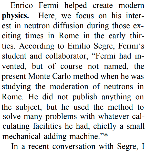
History
- 1946: Stanislaw Ulam, John von Neumann, and Nicholas Metropolis working at Los Alamos National Laboratory develop the Metropolis algorithm.
- 1947: John von Neumann implements the algorithm on the ENIAC computer to simulate neutron diffusion.
- 1953: MCMC algorithms published in the Journal of Chemical Physics.
- 1930s: Enrico Fermi developed a similar method to simulate neutron moderation.
Metropolis-Hastings Algorithm
MH algorithm produces a sequence of samples \({\textcolor{params}{\boldsymbol{\theta}}}^{(1)}, {\textcolor{params}{\boldsymbol{\theta}}}^{(2)}, \ldots, {\textcolor{params}{\boldsymbol{\theta}}}^{(T)}\) that converges to the target distribution \(p({\textcolor{params}{\boldsymbol{\theta}}}\mid {\textcolor{output}{\boldsymbol{y}}})\).
Properties:
- Markov Chain: A sequence of random variables \({\textcolor{params}{\boldsymbol{\theta}}}^{(1)}, {\textcolor{params}{\boldsymbol{\theta}}}^{(2)}, \ldots, {\textcolor{params}{\boldsymbol{\theta}}}^{(T)}\) where the distribution of \({\textcolor{params}{\boldsymbol{\theta}}}^{(t)}\) depends only on \({\textcolor{params}{\boldsymbol{\theta}}}^{(t-1)}\).
- Stationary Distribution: The distribution of \({\textcolor{params}{\boldsymbol{\theta}}}^{(t)}\) converges to the target distribution \(p({\textcolor{params}{\boldsymbol{\theta}}}\mid {\textcolor{output}{\boldsymbol{y}}})\) as \(t \to \infty\).
Metropolis-Hastings Algorithm
How to generate the sequence of samples \({\textcolor{params}{\boldsymbol{\theta}}}^{(1)}, {\textcolor{params}{\boldsymbol{\theta}}}^{(2)}, \ldots, {\textcolor{params}{\boldsymbol{\theta}}}^{(T)}\)?
Initialization: Start with an initial value \({\textcolor{params}{\boldsymbol{\theta}}}^{(1)}\).
Proposal Distribution: Generate a candidate sample \({\textcolor{params}{\boldsymbol{\theta}}}'\) from a proposal distribution \(q({\textcolor{params}{\boldsymbol{\theta}}}' \mid {\textcolor{params}{\boldsymbol{\theta}}}^{(t)})\).
Accepts/Rejects: Accept the candidate sample based on some criteria.
- If accepted, set \({\textcolor{params}{\boldsymbol{\theta}}}^{(t+1)} = {\textcolor{params}{\boldsymbol{\theta}}}'\).
- If rejected, set \({\textcolor{params}{\boldsymbol{\theta}}}^{(t+1)} = {\textcolor{params}{\boldsymbol{\theta}}}^{(t)}\).
Repeat: Repeat steps 2-3 until we have \(T\) samples.
Metropolis-Hastings Algorithm: Proposal Distribution
\(q({\textcolor{params}{\boldsymbol{\theta}}}' \mid {\textcolor{params}{\boldsymbol{\theta}}}^{(t)})\) is a distribution that generates candidate samples \({\textcolor{params}{\boldsymbol{\theta}}}'\) given the current sample \({\textcolor{params}{\boldsymbol{\theta}}}^{(t)}\).
We are free to choose any distribution as the proposal distribution (with the same or larger support as the target distribution).
Symmetric Proposal Distribution: \(q({\textcolor{params}{\boldsymbol{\theta}}}' \mid {\textcolor{params}{\boldsymbol{\theta}}}^{(t)}) = q({\textcolor{params}{\boldsymbol{\theta}}}^{(t)} \mid {\textcolor{params}{\boldsymbol{\theta}}}')\).
Random Walk Proposal: \(q({\textcolor{params}{\boldsymbol{\theta}}}' \mid {\textcolor{params}{\boldsymbol{\theta}}}^{(t)}) = {\mathcal{N}}({\textcolor{params}{\boldsymbol{\theta}}}^{(t)}, {\boldsymbol{\Sigma}})\).
\[ {\boldsymbol{\Sigma}}= \mqty(1 & 0 \\ 0 & 1) \]
\[ {\boldsymbol{\Sigma}}= \mqty(0.1 & 0 \\ 0 & 0.1) \]

Metropolis-Hastings Algorithm: Acceptance Criteria
How to decide whether to accept or reject the candidate sample \({\textcolor{params}{\boldsymbol{\theta}}}'\)?
In the general case, acceptance based on:
\[ \alpha = \frac{p({\textcolor{params}{\boldsymbol{\theta}}}' \mid {\textcolor{output}{\boldsymbol{y}}})p({\textcolor{params}{\boldsymbol{\theta}}}^{(t)} \mid {\textcolor{params}{\boldsymbol{\theta}}}')}{p({\textcolor{params}{\boldsymbol{\theta}}}^{(t)} \mid {\textcolor{output}{\boldsymbol{y}}})p({\textcolor{params}{\boldsymbol{\theta}}}' \mid {\textcolor{params}{\boldsymbol{\theta}}}^{(t)})} \]
If proposal distribution is symmetric,
\[ \alpha = \frac{p({\textcolor{params}{\boldsymbol{\theta}}}' \mid {\textcolor{output}{\boldsymbol{y}}})}{p({\textcolor{params}{\boldsymbol{\theta}}}^{(t)} \mid {\textcolor{output}{\boldsymbol{y}}})} = \frac{p({\textcolor{output}{\boldsymbol{y}}}\mid {\textcolor{params}{\boldsymbol{\theta}}}')p({\textcolor{params}{\boldsymbol{\theta}}}')/Z}{p({\textcolor{output}{\boldsymbol{y}}}\mid {\textcolor{params}{\boldsymbol{\theta}}}^{(t)})p({\textcolor{params}{\boldsymbol{\theta}}}^{(t)})/Z} = \frac{p({\textcolor{output}{\boldsymbol{y}}}\mid {\textcolor{params}{\boldsymbol{\theta}}}')p({\textcolor{params}{\boldsymbol{\theta}}}')}{p({\textcolor{output}{\boldsymbol{y}}}\mid {\textcolor{params}{\boldsymbol{\theta}}}^{(t)})p({\textcolor{params}{\boldsymbol{\theta}}}^{(t)})} \]
Tip
Compute the acceptance ratio in the log-space to be numerically stable.
Metropolis-Hastings Algorithm: Acceptance Criteria
- Acceptance: If \(\alpha \geq 1\), accept the candidate sample \({\textcolor{params}{\boldsymbol{\theta}}}'\).
- Rejection: If \(\alpha < 1\), accept the candidate sample \({\textcolor{params}{\boldsymbol{\theta}}}'\) with probability \(\alpha\).
Intuition:
- If \({\textcolor{params}{\boldsymbol{\theta}}}'\) is more likely than \({\textcolor{params}{\boldsymbol{\theta}}}^{(t)}\), accept \({\textcolor{params}{\boldsymbol{\theta}}}'\).
- If \({\textcolor{params}{\boldsymbol{\theta}}}'\) is less likely than \({\textcolor{params}{\boldsymbol{\theta}}}^{(t)}\), accept \({\textcolor{params}{\boldsymbol{\theta}}}'\) with some probability.
Metropolis-Hastings Algorithm
Steps:
- Initialize \({\textcolor{params}{\boldsymbol{\theta}}}^{(1)}\).
- For \(t = 1, 2, \ldots, T\):
- Generate a candidate sample \({\textcolor{params}{\boldsymbol{\theta}}}' \sim q({\textcolor{params}{\boldsymbol{\theta}}}' \mid {\textcolor{params}{\boldsymbol{\theta}}}^{(t)})\).
- Compute the acceptance ratio \(\alpha\).
- Sample \(u \sim {\mathcal{U}}(0, 1)\).
- Compute \(A = \min(1, \alpha)\).
- Set new sample: \[ {\textcolor{params}{\boldsymbol{\theta}}}^{(t+1)} = \begin{cases} {\textcolor{params}{\boldsymbol{\theta}}}' & \text{if } u \leq A \text{ (accept)}\\ {\textcolor{params}{\boldsymbol{\theta}}}^{(t)} & \text{if } u > A \text{ (reject)} \end{cases} \]
- Repeat step 2 until we have \(T\) samples.
Effect of Proposal Distribution

Assessing Convergence
When to stop?
MCMC algorithms converge to the target distribution as \(T \to \infty\).
Practically, we need to decide when to stop the algorithm or to be able to assess its convergence.
Burn-in Period: Discard the initial samples to allow the chain to converge to the target distribution.
Visual Inspection: Plot the trace of the samples and check for convergence.
Compute heuristics: Compute some metrics to assess convergence.
Burn-in Period and Mixing Time
Burn some initial samples to allow the chain to mix and converge to the target distribution.

Running multiple chains and looking at the trace
Good practice: Run multiple chains from different starting points and plot the trace of the samples.

Running multiple chains and looking at the trace
Good practice: Run multiple chains from different starting points and plot the trace of the samples.

Assessing Convergence with \(\hat{R}\)
Intuition: If multiple chains have converged, in-chain variance should be similar to between-chain variance.
Potential Scale Reduction Factor (\(\hat{R}\)):
\[ \hat{R} = \sqrt{\frac{\text{between-chain variance}}{\text{in-chain variance}}} \]
In practice:
- \(\hat{R} > 1.01\): Some chains have not converged, you may need to run the chains longer.
- \(\hat{R} < 1.01\): Convergence has been reached.
Propose better and accept more
Hamiltonian Monte Carlo
Hamiltonian Monte Carlo (HMC): A more sophisticated MCMC algorithm that uses the concept of Hamiltonian dynamics to propose better samples.
Idea:
Use gradient information to guide local exploration of the target distribution.
Propose samples by simulating the dynamics of a particle moving in a potential energy landscape.
Hamiltonian Dynamics
A particle moving in a potential energy landscape \(\mathcal{U}({\textcolor{params}{\boldsymbol{\theta}}})\) with momentum \(\textcolor{vparams}{{\boldsymbol{\rho}}}\).
Hamiltonian:
\[ \mathcal{H}({\textcolor{params}{\boldsymbol{\theta}}}, \textcolor{vparams}{{\boldsymbol{\rho}}}) = \mathcal{U}({\textcolor{params}{\boldsymbol{\theta}}}) + \mathcal{K}(\textcolor{vparams}{{\boldsymbol{\rho}}}) \]
- \(\mathcal{U}({\textcolor{params}{\boldsymbol{\theta}}})\): Potential energy of the particle at position \({\textcolor{params}{\boldsymbol{\theta}}}\).
- \(\mathcal{K}(\textcolor{vparams}{{\boldsymbol{\rho}}})\): Kinetic energy of the particle with momentum \(\textcolor{vparams}{{\boldsymbol{\rho}}}\).
We consider:
- \(\mathcal{U}({\textcolor{params}{\boldsymbol{\theta}}}) = -\log p({\textcolor{params}{\boldsymbol{\theta}}}\mid {\textcolor{output}{\boldsymbol{y}}})\), where \(p({\textcolor{params}{\boldsymbol{\theta}}}\mid {\textcolor{output}{\boldsymbol{y}}})\) is the target distribution.
- \(\mathcal{K}(\textcolor{vparams}{{\boldsymbol{\rho}}}) = \frac{1}{2}\textcolor{vparams}{{\boldsymbol{\rho}}}{\boldsymbol{M}}^{-1}\textcolor{vparams}{{\boldsymbol{\rho}}}\), where \({\boldsymbol{M}}\) is the mass matrix.
Hamiltonian Dynamics

Energy Conservation
In case of no-friction, the Hamiltonian is conserved.
The trajectory of the particle in the potential energy landscape is governed by the Hamiltonian equations:
\[ \begin{aligned} \frac{\dd {\textcolor{params}{\boldsymbol{\theta}}}}{\dd t} &= \grad_{\textcolor{vparams}{{\boldsymbol{\rho}}}}\mathcal{H}( {\textcolor{params}{\boldsymbol{\theta}}}, \textcolor{vparams}{{\boldsymbol{\rho}}}) = \grad_{\textcolor{vparams}{{\boldsymbol{\rho}}}}\mathcal{K}(\textcolor{vparams}{{\boldsymbol{\rho}}}) \\ \frac{\dd {\color{vparams}{{\boldsymbol{\rho}}}}}{\dd t} &= -\grad_{{\textcolor{params}{\boldsymbol{\theta}}}}\mathcal{H}({\textcolor{params}{\boldsymbol{\theta}}}, \textcolor{vparams}{{\boldsymbol{\rho}}}) = -\grad_{{\textcolor{params}{\boldsymbol{\theta}}}}\mathcal{U}({\textcolor{params}{\boldsymbol{\theta}}}) \end{aligned} \]
The energy is conserved: \(\frac{\dd {{\mathcal{H}}}}{\dd t} = 0\).
Important
To simulate the dynamics of the particle, we don’t need to know the normalization constant \(Z\) for \({\mathcal{U}}({\textcolor{params}{\boldsymbol{\theta}}})= -\log p({\textcolor{params}{\boldsymbol{\theta}}}\mid {\textcolor{output}{\boldsymbol{y}}})\).
Why? Because the dynamics only depend on the gradient of the log-density \(\grad_{{\textcolor{params}{\boldsymbol{\theta}}}}\log p({\textcolor{params}{\boldsymbol{\theta}}}\mid {\textcolor{output}{\boldsymbol{y}}}) = \grad_{{\textcolor{params}{\boldsymbol{\theta}}}}[ \log p({\textcolor{output}{\boldsymbol{y}}}\mid{\textcolor{params}{\boldsymbol{\theta}}}) + \log p({\textcolor{params}{\boldsymbol{\theta}}}) - \log Z]\).
Numerical Solution to the Hamiltonian Equations
\[ \begin{aligned} \frac{\dd {\textcolor{params}{\boldsymbol{\theta}}}}{\dd t} &= \grad_{\textcolor{vparams}{{\boldsymbol{\rho}}}}\mathcal{K}(\textcolor{vparams}{{\boldsymbol{\rho}}}) \\ \frac{\dd {\color{vparams}{{\boldsymbol{\rho}}}}}{\dd t} &= -\grad_{{\textcolor{params}{\boldsymbol{\theta}}}}\mathcal{U}({\textcolor{params}{\boldsymbol{\theta}}}) \end{aligned} \]
Solving exactly is infeasible, but we can use numerical methods to approximate the solution.
Leapfrog Integrator:
Start with \({\textcolor{params}{\boldsymbol{\theta}}}, \textcolor{vparams}{{\boldsymbol{\rho}}}\).
Repeat for \(L\) steps:
- Update momentum: \(\textcolor{vparams}{{\boldsymbol{\rho}}} \leftarrow \textcolor{vparams}{{\boldsymbol{\rho}}} - \frac{\epsilon}{2}\grad_{{\textcolor{params}{\boldsymbol{\theta}}}}\mathcal{U}({\textcolor{params}{\boldsymbol{\theta}}})\).
- Update position: \({\textcolor{params}{\boldsymbol{\theta}}}\leftarrow {\textcolor{params}{\boldsymbol{\theta}}}+ \epsilon \grad_{\textcolor{vparams}{{\boldsymbol{\rho}}}}\mathcal{K}(\textcolor{vparams}{{\boldsymbol{\rho}}})\).
- Update momentum: \(\textcolor{vparams}{{\boldsymbol{\rho}}} \leftarrow \textcolor{vparams}{{\boldsymbol{\rho}}} - \frac{\epsilon}{2}\grad_{{\textcolor{params}{\boldsymbol{\theta}}}}\mathcal{U}({\textcolor{params}{\boldsymbol{\theta}}})\).
Equilibrium with Energy Conservation

Simulating Hamiltonian Dynamics \(\Leftrightarrow\) Sampling
\[ p({\textcolor{params}{\boldsymbol{\theta}}}, {\color{vparams}{{\boldsymbol{\rho}}}}) = \frac 1 {Z_H} \exp(-\mathcal{H}({\textcolor{params}{\boldsymbol{\theta}}}, {\color{vparams}{{\boldsymbol{\rho}}}})) = \frac 1{Z_H} \exp\left(-\mathcal{U}({\textcolor{params}{\boldsymbol{\theta}}}) - \frac{1}{2}{\color{vparams}{{\boldsymbol{\rho}}}}^\top{\boldsymbol{M}}^{-1}{\color{vparams}{{\boldsymbol{\rho}}}}\right) \]
The marginal distribution of \({\textcolor{params}{\boldsymbol{\theta}}}\) is the target distribution \(p({\textcolor{params}{\boldsymbol{\theta}}}\mid {\textcolor{output}{\boldsymbol{y}}})\).
\[ p({\textcolor{params}{\boldsymbol{\theta}}}\mid {\textcolor{output}{\boldsymbol{y}}}) = \int p({\textcolor{params}{\boldsymbol{\theta}}}, {\color{vparams}{{\boldsymbol{\rho}}}}) \dd {\color{vparams}{{\boldsymbol{\rho}}}} = \frac{1}{Z} \exp(-\mathcal{U}({\textcolor{params}{\boldsymbol{\theta}}}))\frac{1}{Z_K}\int \exp\left(-\frac{1}{2}{\color{vparams}{{\boldsymbol{\rho}}}}^\top{\boldsymbol{M}}^{-1}{\color{vparams}{{\boldsymbol{\rho}}}}\right)\dd {\color{vparams}{{\boldsymbol{\rho}}}} = \frac{1}{Z} \exp(-\mathcal{U}({\textcolor{params}{\boldsymbol{\theta}}})) \]
Hamiltonian Monte Carlo Algorithm
Suppose the last sample in the sequence is \({\textcolor{params}{\boldsymbol{\theta}}}^{(t-1)}\)
- Initialization:
- Set \({\textcolor{params}{\boldsymbol{\theta}}}^\prime_0 = {\textcolor{params}{\boldsymbol{\theta}}}^{(t-1)}\).
- Sample momentum \(\textcolor{vparams}{{\boldsymbol{\rho}}}^\prime_0 \sim {\mathcal{N}}(0, {\boldsymbol{M}})\).
- Hamiltonian Dynamics:
- Simulate Hamiltonian dynamics for \(L\) steps to obtain \({\textcolor{params}{\boldsymbol{\theta}}}^\prime_L, \textcolor{vparams}{{\boldsymbol{\rho}}}^\prime_L\).
- Acceptance:
- Accept with probability \(\alpha\)
\[ \alpha = \min\left(1, \frac{p({\textcolor{params}{\boldsymbol{\theta}}}^\prime_L, \textcolor{vparams}{{\boldsymbol{\rho}}}^\prime_L)}{p({\textcolor{params}{\boldsymbol{\theta}}}^{(t-1)}, \textcolor{vparams}{{\boldsymbol{\rho}}}^{(t-1)})}\right) = \min\left(1, \exp\left(-\mathcal{H}({\textcolor{params}{\boldsymbol{\theta}}}^\prime_L, \textcolor{vparams}{{\boldsymbol{\rho}}}^\prime_L) + \mathcal{H}({\textcolor{params}{\boldsymbol{\theta}}}^{(t-1)}, \textcolor{vparams}{{\boldsymbol{\rho}}}^{(t-1)})\right)\right) \]
Tuning HMC
- Number of Steps: The number of steps \(L\) to simulate the Hamiltonian dynamics.
- Step Size: The size of the leapfrog steps \(\epsilon\).
- Mass Matrix: The mass matrix \({\boldsymbol{M}}\).
Considerations:
- \(L\) needs to be large enough to explore the target distribution, but small enough to avoid wasting computation.
- \(\epsilon\) needs to be small enough to avoid numerical instability, but large enough to have \(\alpha\) close to 1.
- \({\boldsymbol{M}}\) can be set to the identity matrix or estimated from the target distribution (after burn-in).
Extensions of HMC
No-U-Turn Sampler (NUTS): Automatically adapt the number of steps \(L\).
Stochastic Gradient Hamiltonian Monte Carlo: Use stochastic gradients to scale to large datasets
\[ \begin{aligned} {\mathcal{U}}({\textcolor{params}{\boldsymbol{\theta}}}) &= -\log p({\textcolor{params}{\boldsymbol{\theta}}}\mid {\textcolor{output}{\boldsymbol{y}}}) \propto -\sum_{i=1}^n \log p({\textcolor{output}{\boldsymbol{y}}}_i \mid {\textcolor{params}{\boldsymbol{\theta}}}) - \log p({\textcolor{params}{\boldsymbol{\theta}}})\\ \end{aligned} \]
Applications
Sampling from a language model efficiently
Generate new data with diffusion models
Source: Score-Based Generative Modeling with Critically-Damped Langevin Diffusion
![]()
Simone Rossi - Advanced Statistical Inference - EURECOM