Neural Networks: A probabilistic perspective

Advanced Statistical Inference

Simone Rossi

EURECOM

Neural Networks and Deep Learning

\[ \require{physics} \definecolor{input}{rgb}{0.42, 0.55, 0.74} \definecolor{params}{rgb}{0.51,0.70,0.40} \definecolor{output}{rgb}{0.843, 0.608, 0} \definecolor{vparams}{rgb}{0.58, 0, 0.83} \definecolor{noise}{rgb}{0.0, 0.48, 0.65} \definecolor{latent}{rgb}{0.8, 0.0, 0.8} \]

Deep learning has changed the scale of problems we can solve with machine learning.

Protein folding

Chip design

Introduction

Neural networks are a class of parametric models that are widely used in machine learning and statistics.
Build complex functions by composing simple functions.

\[ \begin{aligned} \textcolor{latent}{f}= \textcolor{latent}{f}_L \circ \textcolor{latent}{f}_{L-1} \circ \ldots \circ \textcolor{latent}{f}_1 \end{aligned} \]

Composition of functions

Generally, each function \(\textcolor{latent}{f}_i\) is a linear transformation followed by a non-linear activation function.

For example, in a feedforward MLP: \[ \textcolor{latent}{f}_i({\textcolor{params}{\boldsymbol{\theta}}}_i, {\textcolor{input}{\boldsymbol{x}}}) = a({\textcolor{params}{\boldsymbol{W}}}_i {\textcolor{input}{\boldsymbol{x}}}+ {\textcolor{params}{\boldsymbol{b}}}_i) \]

where \({\textcolor{params}{\boldsymbol{W}}}_i\) is a matrix of weights, \({\textcolor{params}{\boldsymbol{b}}}_i\) is a bias vector, and \(a(\cdot)\) is the activation function.

Neural Networks: Architectures

From linear models to neural networks

From a probabilistic perspective, we still need to define a likelihood:

Regression with noisy outputs: Gaussian likelihood \[ p({\textcolor{output}{\boldsymbol{y}}}\mid{\textcolor{params}{\boldsymbol{\theta}}}) = \prod_{i=1}^N {\mathcal{N}}(\textcolor{output}{y}_i\mid \textcolor{latent}{f}({\textcolor{params}{\boldsymbol{\theta}}}, {\textcolor{input}{\boldsymbol{x}}}_i), \sigma^2) \]
Binary classification: Bernoulli likelihood \[ p({\textcolor{output}{\boldsymbol{y}}}\mid{\textcolor{params}{\boldsymbol{\theta}}}) = \prod_{i=1}^N \text{Bern}(\textcolor{output}{y}_i\mid \sigma(\textcolor{latent}{f}({\textcolor{params}{\boldsymbol{\theta}}}, {\textcolor{input}{\boldsymbol{x}}}_i))) \]
Multi-class classification: Categorical likelihood \[ p({\textcolor{output}{\boldsymbol{y}}}\mid{\textcolor{params}{\boldsymbol{\theta}}}) = \prod_{i=1}^N \text{Cat}(\textcolor{output}{y}_i\mid \text{sfmx}(\textcolor{latent}{f}({\textcolor{params}{\boldsymbol{\theta}}}, {\textcolor{input}{\boldsymbol{x}}}_i))) \]

Training neural networks

Training neural networks involves optimizing the parameters \({\textcolor{params}{\boldsymbol{\theta}}}\) to maximize the likelihood of the data.

\[ {\textcolor{params}{\boldsymbol{\theta}}}^* = \arg\max_{{\textcolor{params}{\boldsymbol{\theta}}}} p({\textcolor{output}{\boldsymbol{y}}}\mid{\textcolor{params}{\boldsymbol{\theta}}}) \]

This is typically done by using the backpropagation algorithm
The backpropagation algorithm computes the gradient with respect to the parameters \({\textcolor{params}{\boldsymbol{\theta}}}\) using the chain rule

\[ \begin{aligned} \frac{\partial \log p({\textcolor{output}{\boldsymbol{y}}}\mid{\textcolor{params}{\boldsymbol{\theta}}})}{\partial {\textcolor{params}{\boldsymbol{\theta}}}_i} = \frac{\partial \log p({\textcolor{output}{\boldsymbol{y}}}\mid{\textcolor{params}{\boldsymbol{\theta}}})}{\partial \textcolor{latent}{f}_L} \frac{\partial \textcolor{latent}{f}_L}{\partial \textcolor{latent}{f}_{L-1}} \ldots \frac{\partial \textcolor{latent}{f}_{i+1}}{\partial {\textcolor{params}{\boldsymbol{\theta}}}_i} \end{aligned} \]

Training neural networks

The gradient is used to update the parameters using an optimization algorithm (e.g., SGD, Adam)

For SGD, the update rule is:

\[ \begin{aligned} {\textcolor{params}{\boldsymbol{\theta}}}\gets {\textcolor{params}{\boldsymbol{\theta}}}+ \eta \grad_{{\textcolor{params}{\boldsymbol{\theta}}}} \log p({\textcolor{output}{\boldsymbol{y}}}\mid{\textcolor{params}{\boldsymbol{\theta}}}) \end{aligned} \]

where \(\eta\) is the learning rate.

More complex optimization algorithms involve momentum, adaptive learning rates, etc.

Landscape of neural networks

Training neural networks

Optimization of neural networks is a non-convex optimization problem, with many local minima.
Overfitting is a common problem in neural networks, especially when the number of parameters is large.
Common techniques to prevent overfitting include:
- Weight decay
- Dropout

Weight decay is a Gaussian prior

Weight decay is a regularization technique that changes the update rule to:

where \(\lambda\) is the weight decay parameter.

\[ \begin{aligned} \eta \grad_{{\textcolor{params}{\boldsymbol{\theta}}}} \log p({\textcolor{output}{\boldsymbol{y}}}\mid{\textcolor{params}{\boldsymbol{\theta}}}) + \lambda {\textcolor{params}{\boldsymbol{\theta}}}= \eta \left( \grad_{{\textcolor{params}{\boldsymbol{\theta}}}} \log p({\textcolor{output}{\boldsymbol{y}}}\mid{\textcolor{params}{\boldsymbol{\theta}}}) - \frac{\lambda}{\eta} {\textcolor{params}{\boldsymbol{\theta}}}\right) \\ \eta \left( \grad_{{\textcolor{params}{\boldsymbol{\theta}}}} \log p({\textcolor{output}{\boldsymbol{y}}}\mid{\textcolor{params}{\boldsymbol{\theta}}}) + \grad_{{\textcolor{params}{\boldsymbol{\theta}}}} \left( -\frac{\lambda}{\eta} {\textcolor{params}{\boldsymbol{\theta}}}^T {\textcolor{params}{\boldsymbol{\theta}}}\right) \right) \end{aligned} \]

but \(\log {\mathcal{N}}({\textcolor{params}{\boldsymbol{\theta}}}\mid {\boldsymbol{0}}, \frac{\eta}{2\lambda}{\boldsymbol{I}}) \propto -\frac{\lambda}{\eta} {\textcolor{params}{\boldsymbol{\theta}}}^T {\textcolor{params}{\boldsymbol{\theta}}}\)

Important note

Weight decay is equivalent to placing a Gaussian prior on the weights, but the variance of the prior also depends on the learning rate.

Gaussian prior on the weights

The Gaussian prior on the weights can be interpreted as a form of Bayesian regularization.
When we have a weight decay term, the optimization problem is equivalent to maximizing the posterior distribution of the weights.

\[ \begin{aligned} {\textcolor{params}{\boldsymbol{\theta}}}^* = \arg\max_{{\textcolor{params}{\boldsymbol{\theta}}}} p({\textcolor{params}{\boldsymbol{\theta}}}\mid{\textcolor{output}{\boldsymbol{y}}}) = \arg\max_{{\textcolor{params}{\boldsymbol{\theta}}}} p({\textcolor{output}{\boldsymbol{y}}}\mid{\textcolor{params}{\boldsymbol{\theta}}}) p({\textcolor{params}{\boldsymbol{\theta}}}) = \arg\max_{{\textcolor{params}{\boldsymbol{\theta}}}} \left [\log p({\textcolor{output}{\boldsymbol{y}}}\mid{\textcolor{params}{\boldsymbol{\theta}}}) + \log p({\textcolor{params}{\boldsymbol{\theta}}}) \right] \end{aligned} \]

Dropout

Dropout is a technique that randomly sets a fraction of the activations to zero during training.

Dropout formulation

With dropout, during training the output of a layer is given by:

\[ \begin{aligned} {\boldsymbol{z}}\sim \text{Bern}(p) \\ \widetilde {\textcolor{input}{\boldsymbol{x}}}= {\boldsymbol{z}}\odot {\textcolor{input}{\boldsymbol{x}}}\\ {\boldsymbol{h}}= a({\textcolor{params}{\boldsymbol{W}}}\widetilde {\textcolor{input}{\boldsymbol{x}}}+ {\textcolor{params}{\boldsymbol{b}}}) \end{aligned} \]

where \({\boldsymbol{r}}\) is a binary mask, \(p\) is the dropout probability, and \(\odot\) is the element-wise product. At test time, the activations are scaled by \(p\) to account for the fact that more units are active during training.

Note: Dropping out activations can be interpreted as dropping out rows of the weight matrix \({\textcolor{params}{\boldsymbol{W}}}\).

Double descent phenomenon

Neural networks are highly overparametrized models, and they can fit the training data perfectly.
However, they can also generalize well to unseen data.
But the behavior of the generalization error is more complex: this is called the double descent phenomenon.

Bayesian Neural Networks

Bayesian neural networks are neural networks that are trained using a Bayesian approach.

It follows the classic recipe of Bayesian inference:

Define a prior distribution over the parameters \({\textcolor{params}{\boldsymbol{\theta}}}\) (e.g., Gaussian on weights and biases).
Define a likelihood function \(p({\textcolor{output}{\boldsymbol{y}}}\mid{\textcolor{params}{\boldsymbol{\theta}}})\).
Compute the posterior distribution \(p({\textcolor{params}{\boldsymbol{\theta}}}\mid{\textcolor{output}{\boldsymbol{y}}})\).

Problem: The posterior distribution is intractable for neural networks, we need to approximate it.

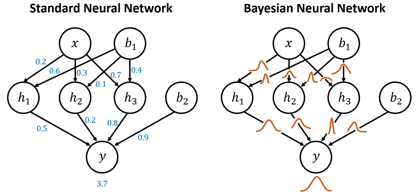
Bayesian Neural Networks

Approximate inference in Bayesian neural networks

We have seens several methods to approximate intractable posterior distributions:

Variational inference
MCMC
Laplace approximation

Everything we have seen so far can be applied to Bayesian neural networks.

But neural networks have particular properties that make them challenging to approximate:

High-dimensional parameter space
Non-convex optimization landscape => non-Gaussian posteriors
Many symmetries => many local minima => multimodal posteriors
Computationally expensive likelihood evaluations
Priors are difficult to specify

Approximate inference in Bayesian neural networks

Let’s focus on three different problems:

Specifying good priors for Bayesian neural networks
Reusing some techniques from neural networks to approximate the posterior (e.g., dropout, ensembles)
Using Gaussian processes to approximate the posterior

Specifying priors for Bayesian neural networks

The choice of prior is crucial in Bayesian inference, as it encodes our prior beliefs about the parameters.
For neural networks, the choice of prior is not straightforward, as the parameters are high-dimensional and they are difficult to interpret.

Specifying priors for Bayesian neural networks

Gaussian prior: the most common choice, can be different for weights and biases. It has a close connection with weight decay.

\[ \begin{aligned} p({\textcolor{params}{\boldsymbol{\theta}}}) = \prod_{i=1}^L {\mathcal{N}}({\textcolor{params}{\boldsymbol{\theta}}}_i\mid 0, \sigma^2) \end{aligned} \]

Laplace prior: can be used to promote sparsity in the weights.
Scale mixture prior: can be used to promote heavy-tailed distributions.

\[ \begin{aligned} p({\textcolor{params}{\boldsymbol{\theta}}}) = \prod_{i=1}^L {\mathcal{N}}({\textcolor{params}{\boldsymbol{\theta}}}_i\mid 0, \sigma^2) \quad \text{with} \quad \sigma^2 \sim p(\sigma^2) \end{aligned} \]

where \(p(\sigma^2)\) can be a Gamma, Inverse-Gamma, Exponential, or other distributions.

Dropout as a Bayesian approximation

Idea: Instead of applying dropout only during training, we can sample from the dropout mask at test time many times and use the ensemble of predictions.

This is called Monte Carlo dropout.

Dropout as a Bayesian approximation

Dropout can be interpreted as a form of variational inference.

\[ {\mathcal{L}}_{\text{ELBO}}= {\mathbb{E}}_{q({\textcolor{params}{\boldsymbol{\theta}}})}[\log p({\textcolor{output}{\boldsymbol{y}}}\mid{\textcolor{params}{\boldsymbol{\theta}}})] - \text{KL}\left(q({\textcolor{params}{\boldsymbol{\theta}}}) \parallel p({\textcolor{params}{\boldsymbol{\theta}}})\right) \]

where \(q({\textcolor{params}{\boldsymbol{\theta}}})\) is the variational distribution, and \(p({\textcolor{params}{\boldsymbol{\theta}}})\) is the prior.

For MC dropout with dropout probability \(p\), the variational distribution is:

\[ q({\textcolor{params}{\boldsymbol{\theta}}}) = (1-p) {\mathcal{N}}({\boldsymbol{m}}, {\boldsymbol{\sigma}}^2) + p {\mathcal{N}}({\boldsymbol{0}}, {\boldsymbol{\sigma}}^2) \]

Note: The KL divergence is not tractable analytically, but it can be approximated using the Monte Carlo method.

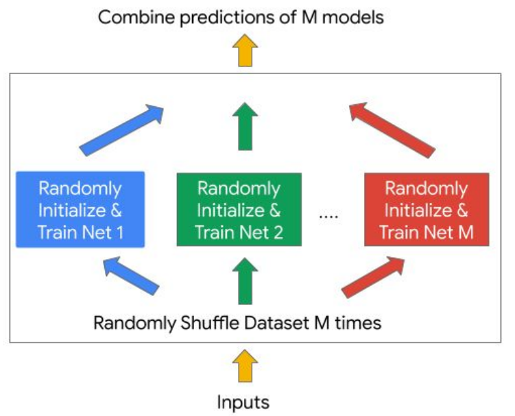
Deep ensembles

Idea: Train multiple neural networks independently with different initializations and average their predictions.

Advantages:
- Deep ensemble methods are easy to implement and training is highly parallelizable.
- They can be used with any neural network architecture, loss function, and optimization algorithm
- They can be used to estimate the uncertainty of the predictions.

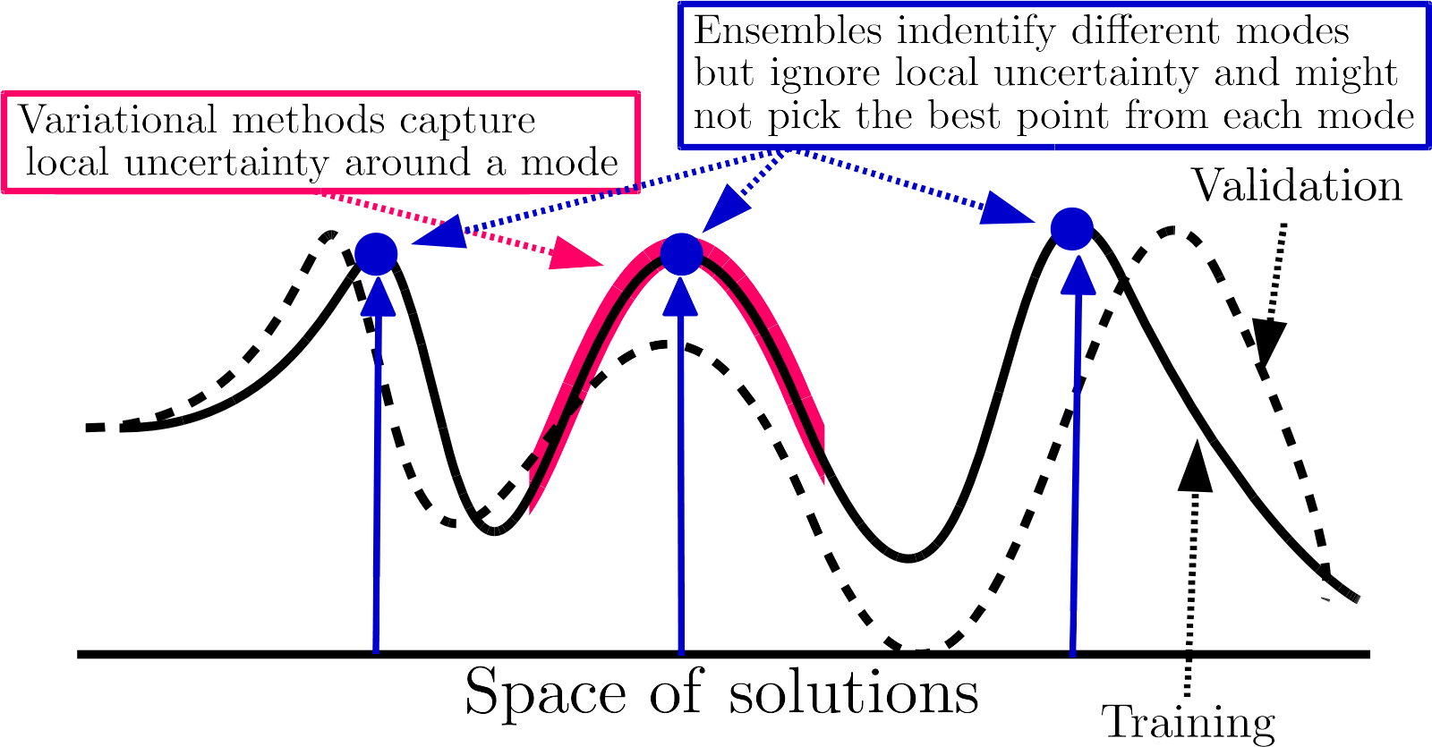
Why do deep ensembles work? An intuitive explanation

Diversity: each neural network is trained with a different initialization, so they will converge to different local minima, separating the modes of the posterior distribution.

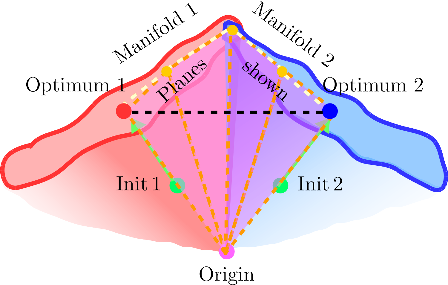
Connecting the modes of the posterior distribution

Why do deep ensembles work?

Under some assumptions, deep ensembles can be interpreted as a form of approximate Bayesian inference.

Theoretical connections between neural networks and kernel methods

Behaviour of wide neural networks

Some interesting insights from Radford M. Neal’s 1993 thesis:

Gaussian processes are a powerful tool for machine learning
Neural networks are universal function approximators and they can generalize well despite overparametrization
The infinite-width limit of neural networks is a Gaussian process

Infinite-width neural networks

Consider a single hidden layer neural network: \[ {\textcolor{latent}{\boldsymbol{f}}}({\textcolor{params}{\boldsymbol{\theta}}}, {\textcolor{input}{\boldsymbol{x}}}) = {\textcolor{params}{\boldsymbol{w}}}^\top a({\textcolor{params}{\boldsymbol{W}}}{\textcolor{input}{\boldsymbol{x}}}+ {\textcolor{params}{\boldsymbol{b}}}) \] where \({\textcolor{params}{\boldsymbol{W}}}\in{\mathbb{R}}^{M\times D}\), \({\textcolor{params}{\boldsymbol{w}}}\in {\mathbb{R}}^M\), \({\textcolor{params}{\boldsymbol{b}}}\in {\mathbb{R}}^M\) and \(a(\cdot)\) is the activation function.
In the limit of infinite width (\(M\to\infty\)), randomly initialized neural networks becomes a Gaussian process, regardless of the choice of activation function.

Infinite-width neural networks

Remember the definition of a Gaussian process:

A Gaussian process is a collection of random variables, with some index set, such that any finite subset of the random variables has a joint Gaussian distribution.

\[ \textcolor{latent}{f}({\textcolor{input}{\boldsymbol{x}}}_1), \textcolor{latent}{f}({\textcolor{input}{\boldsymbol{x}}}_2), \ldots, \textcolor{latent}{f}({\textcolor{input}{\boldsymbol{x}}}_N) \sim {\mathcal{N}}({\boldsymbol{0}}, {\boldsymbol{K}}) \]

where \({\boldsymbol{K}}_{ij} = k({\textcolor{input}{\boldsymbol{x}}}_i, {\textcolor{input}{\boldsymbol{x}}}_j)\) is the covariance matrix computed using the kernel function \(k(\cdot, \cdot)\).

Infinite-width neural networks

Depending on the choice of activation function, the infinite-width neural network can be interpreted as a Gaussian process with a specific kernel.

Activation function	Finite-limit Kernel
ReLU	Arc-cosine kernel \(k({\textcolor{input}{\boldsymbol{x}}}, {\textcolor{input}{\boldsymbol{x}}}^\prime) = \frac{\norm{{\textcolor{input}{\boldsymbol{x}}}}\norm{{\textcolor{input}{\boldsymbol{x}}}^\prime}}{2\pi} \left( \sin \theta + (\pi - \theta) \cos \theta \right)\) with \(\theta = \cos^{-1} \left( \frac{{\textcolor{input}{\boldsymbol{x}}}^\top {\textcolor{input}{\boldsymbol{x}}}^\prime}{\norm{{\textcolor{input}{\boldsymbol{x}}}}\norm{{\textcolor{input}{\boldsymbol{x}}}^\prime}} \right)\)
Trigonometric (sin/cos)	Squared exponential or RBF kernel \(k({\textcolor{input}{\boldsymbol{x}}}, {\textcolor{input}{\boldsymbol{x}}}^\prime) = \exp\left( -\frac{\norm{{\textcolor{input}{\boldsymbol{x}}}- {\textcolor{input}{\boldsymbol{x}}}^\prime}^2}{2\ell^2} \right)\)

ReLU

Arc-cosine kernel \(k({\textcolor{input}{\boldsymbol{x}}}, {\textcolor{input}{\boldsymbol{x}}}^\prime) = \frac{\norm{{\textcolor{input}{\boldsymbol{x}}}}\norm{{\textcolor{input}{\boldsymbol{x}}}^\prime}}{2\pi} \left( \sin \theta + (\pi - \theta) \cos \theta \right)\) with \(\theta = \cos^{-1} \left( \frac{{\textcolor{input}{\boldsymbol{x}}}^\top {\textcolor{input}{\boldsymbol{x}}}^\prime}{\norm{{\textcolor{input}{\boldsymbol{x}}}}\norm{{\textcolor{input}{\boldsymbol{x}}}^\prime}} \right)\)

Trigonometric (sin/cos)

Squared exponential or RBF kernel \(k({\textcolor{input}{\boldsymbol{x}}}, {\textcolor{input}{\boldsymbol{x}}}^\prime) = \exp\left( -\frac{\norm{{\textcolor{input}{\boldsymbol{x}}}- {\textcolor{input}{\boldsymbol{x}}}^\prime}^2}{2\ell^2} \right)\)

Infinite-width neural networks

So far, we have seen that one-hidden layer neural networks can be interpreted as Gaussian processes in the infinite-width limit.

But during the years, many other results have been obtained for more complex architectures:
- G. de G. Matthews, et al. “Gaussian Process Behaviour in Wide Deep Neural Networks”. ICLR 2018.
- J. Lee, et al. “Deep Neural Networks as Gaussian Processes”. ICLR 2018.
- A. Novak, et al. “Bayesian Deep Convolutional Networks with Many Channels are Gaussian Processes”. NeurIPS 2018.
- A. Garriga-Alonso, et al. “Deep convolutional networks as shallow Gaussian processes”. ICLR 2019.
- G. Yang, et al. “Wide Feedforward or Recurrent Neural Networks of Any Architecture are Gaussian Processes”. NeurIPS 2019.

Infinite-width neural networks

The main idea is that as the width of the network increases, the output of randomly initialized neural networks \(\textcolor{latent}{f}_0({\textcolor{input}{\boldsymbol{x}}})\) converges to a Gaussian process.

\[ \textcolor{latent}{f}_0({\textcolor{input}{\boldsymbol{x}}}) \sim {\mathcal{N}}({\boldsymbol{0}}, {\boldsymbol{K}}) \quad \text{with} \quad {\boldsymbol{K}}= \lim_{M\to\infty} {\mathbb{E}}[{\textcolor{latent}{\boldsymbol{f}}}_0({\textcolor{input}{\boldsymbol{x}}}) {\textcolor{latent}{\boldsymbol{f}}}_0({\textcolor{input}{\boldsymbol{x}}})^\top] \]

Infinite-width neural networks

Controversial opinions on infinite-width neural networks:

Pro:
- Infinite-width limits be used to derive theoretical results for deep learning.
- They can be used to design better optimization algorithms.
- They can be used to design better architectures.

Con:
- Feature-learning is one of the main advantages of neural networks, but in the infinite-width limit there are no features to learn.

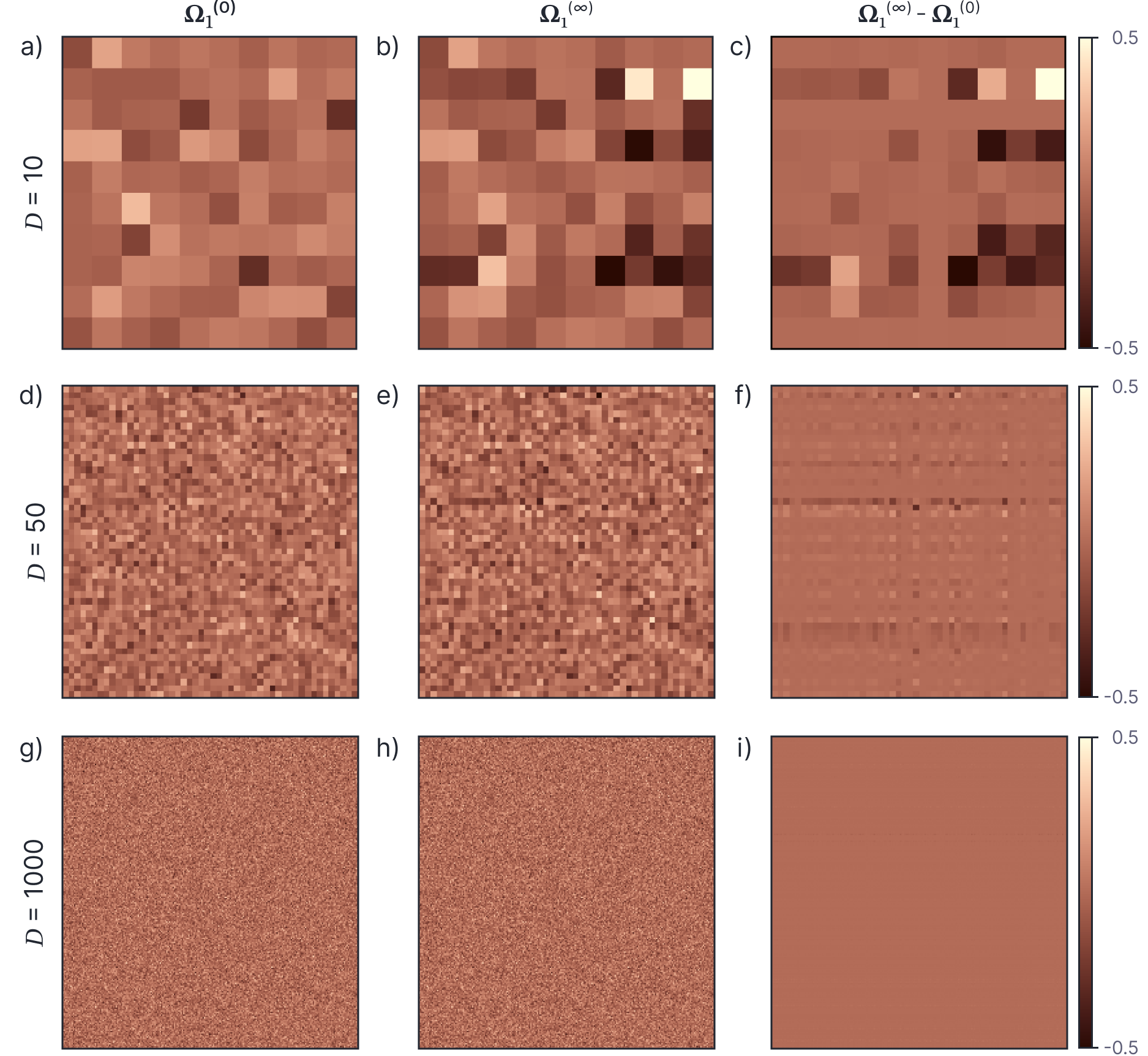
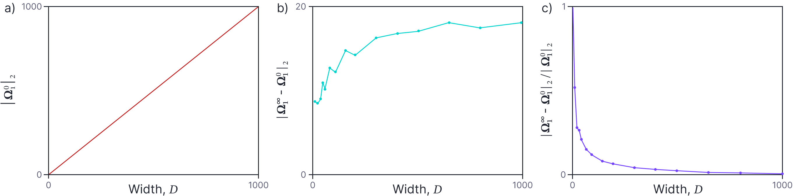
Wide neural networks don’t learn features

Change in weights of a 2 layer neural network as the number of features increases.

The norm of the initial weight matrix increases as the number of features increases.
The norm of the change in weights is roughly constant as the number of features increases.
The norm of the change relative to the initial norm decreases with the number of features.

Neural Tangent Kernel

Bayesian inference and the GP limit give a lot of insights into the behaviour of overparametrized neural networks.
However, the GP limit is not practical for training neural networks.
Can we apply a similar interpretation to finite-width neural networks trained with gradient descent?
- Goal: analyze the dynamics of gradient-based optimization in finite-width neural networks.

Gradient flow

Start from the gradient descent update rule:

\[ \begin{aligned} {\textcolor{params}{\boldsymbol{\theta}}}_{t+1} = {\textcolor{params}{\boldsymbol{\theta}}}_{t} - \eta \grad_{{\textcolor{params}{\boldsymbol{\theta}}}} {\mathcal{L}}({\textcolor{latent}{\boldsymbol{f}}}_{t}, {\textcolor{output}{\boldsymbol{y}}}) \end{aligned} \]

where \({\textcolor{latent}{\boldsymbol{f}}}_{t} = {\textcolor{latent}{\boldsymbol{f}}}({\textcolor{params}{\boldsymbol{\theta}}}_{t}, {\textcolor{input}{\boldsymbol{X}}})\) and \({\mathcal{L}}({\textcolor{latent}{\boldsymbol{f}}}_t, {\textcolor{output}{\boldsymbol{y}}})\) is the loss function.

Re-arrranging terms:

\[ \begin{aligned} \frac{{\textcolor{params}{\boldsymbol{\theta}}}_{t+1} - {\textcolor{params}{\boldsymbol{\theta}}}_{t}}{\eta} = -\grad_{{\textcolor{params}{\boldsymbol{\theta}}}} {\mathcal{L}}({\textcolor{latent}{\boldsymbol{f}}}_{t}, {\textcolor{output}{\boldsymbol{y}}}) \end{aligned} \]

Taking the limit \(\eta \to 0\):

Gradient flow

This is an ordinary differential equation (ODE) that describes the evolution of the parameters \({\textcolor{params}{\boldsymbol{\theta}}}_t\).
\({\textcolor{params}{\boldsymbol{\theta}}}_t\) is a function of time (as in optimization steps)
The solution of this system is called the gradient flow.

If we know the solution of the gradient flow \({\textcolor{params}{\boldsymbol{\theta}}}_t\), for any time \(t\), we can can choose a \(T\) large enough such that \({\textcolor{params}{\boldsymbol{\theta}}}_T\) is close to the minimum of the loss function.

Gradient Flow vs Gradient Descent

Gradient flow in function space

\[ \frac{\dd {\textcolor{params}{\boldsymbol{\theta}}}_t}{\dd t} = -\grad_{{\textcolor{params}{\boldsymbol{\theta}}}} {\mathcal{L}}({\textcolor{latent}{\boldsymbol{f}}}_t, {\textcolor{output}{\boldsymbol{y}}}) \]

Let’s apply chain rule to the gradient of the loss function:

\[ \begin{aligned} \frac{\dd {\textcolor{params}{\boldsymbol{\theta}}}_t}{\dd t} = -\grad_{{\textcolor{params}{\boldsymbol{\theta}}}} {\mathcal{L}}({\textcolor{latent}{\boldsymbol{f}}}_t, {\textcolor{output}{\boldsymbol{y}}}) = -\grad_{{\textcolor{params}{\boldsymbol{\theta}}}} {\textcolor{latent}{\boldsymbol{f}}}_t\grad_{{\textcolor{latent}{\boldsymbol{f}}}} {\mathcal{L}}({\textcolor{latent}{\boldsymbol{f}}}_t, {\textcolor{output}{\boldsymbol{y}}}) \end{aligned} \]

How does \({\textcolor{latent}{\boldsymbol{f}}}\) evolve with time?

\[ \begin{aligned} \frac{\dd {\textcolor{latent}{\boldsymbol{f}}}_t}{\dd t} = \grad_{{\textcolor{params}{\boldsymbol{\theta}}}} {\textcolor{latent}{\boldsymbol{f}}}_t^ \top \frac{\dd {\textcolor{params}{\boldsymbol{\theta}}}_t}{\dd t} \end{aligned} \]

This is the linearized version of the neural network around the current parameters.

\[ {\textcolor{latent}{\boldsymbol{f}}}_{t} \approx {\textcolor{latent}{\boldsymbol{f}}}_{0} + \grad_{{\textcolor{params}{\boldsymbol{\theta}}}} {\textcolor{latent}{\boldsymbol{f}}}_{0}^\top ({\textcolor{params}{\boldsymbol{\theta}}}_t - {\textcolor{params}{\boldsymbol{\theta}}}_0) \]

Neural Tangent Kernel

By combining the two equations, we can obtain the evolution of the neural network in function space:

\[ \frac{\dd {\textcolor{latent}{\boldsymbol{f}}}_t}{\dd t} = -\grad_{{\textcolor{params}{\boldsymbol{\theta}}}} {\textcolor{latent}{\boldsymbol{f}}}_t^\top \grad_{{\textcolor{params}{\boldsymbol{\theta}}}} {\textcolor{latent}{\boldsymbol{f}}}_t \grad_{{\textcolor{latent}{\boldsymbol{f}}}} {\mathcal{L}}({\textcolor{latent}{\boldsymbol{f}}}_t, {\textcolor{output}{\boldsymbol{y}}}) = -{\boldsymbol{\Theta}}_t \grad_{{\textcolor{latent}{\boldsymbol{f}}}} {\mathcal{L}}({\textcolor{latent}{\boldsymbol{f}}}_t, {\textcolor{output}{\boldsymbol{y}}}) \]

where \({\boldsymbol{\Theta}}_t = \grad_{{\textcolor{params}{\boldsymbol{\theta}}}} {\textcolor{latent}{\boldsymbol{f}}}_t^\top \grad_{{\textcolor{params}{\boldsymbol{\theta}}}} {\textcolor{latent}{\boldsymbol{f}}}_t\) is the Neural Tangent Kernel (NTK).

\({\boldsymbol{\Theta}}_t\) is a \(N\times N\) matrix
Generally, \({\boldsymbol{\Theta}}_t\) is a function of the input data \({\textcolor{input}{\boldsymbol{X}}}\) and the parameters \({\textcolor{params}{\boldsymbol{\theta}}}_t\).
When the width of the network is infinite, \({\boldsymbol{\Theta}}_t\) converges to a constant matrix \({\boldsymbol{\Theta}}\), which is independent of the parameters \({\textcolor{params}{\boldsymbol{\theta}}}_t\).

Neural Tangent Kernel as a kernel for Gaussian Processes

The Neural Tangent Kernel is a kernel that describes the evolution of the neural network in function space.
Infinitely-wide neural networks open up ways to study deep neural networks both under fully Bayesian training through the Gaussian process correspondence, and under GD training through the linearization perspective
We can use the NTK as a kernel for Gaussian processes, and use it to make predictions on a test set \({\textcolor{input}{\boldsymbol{x}}}_\star\)

\[ \begin{aligned} {\textcolor{latent}{\boldsymbol{f}}}({\textcolor{input}{\boldsymbol{x}}}_{\star}) \mid {\textcolor{output}{\boldsymbol{y}}}, {\textcolor{input}{\boldsymbol{X}}}\sim {\mathcal{N}}(&{\boldsymbol{\Theta}}_\star {\boldsymbol{\Theta}}^{-1} {\textcolor{output}{\boldsymbol{y}}}, {\boldsymbol{\Theta}}_{\star\star} - {\boldsymbol{\Theta}}_\star {\boldsymbol{\Theta}}^{-1} {\boldsymbol{\Theta}}_\star^\top) % \mbTheta_{\star\star} + \mbTheta_\star \mbTheta^{-1} \mbK\mbTheta^{-1} \mbTheta_\star^\top - (\mbTheta_\star \mbTheta^{-1} \mbK_\star^\top + \mbTheta_\star^\top \mbTheta^{-1} \mbK_\star) ) \end{aligned} \]

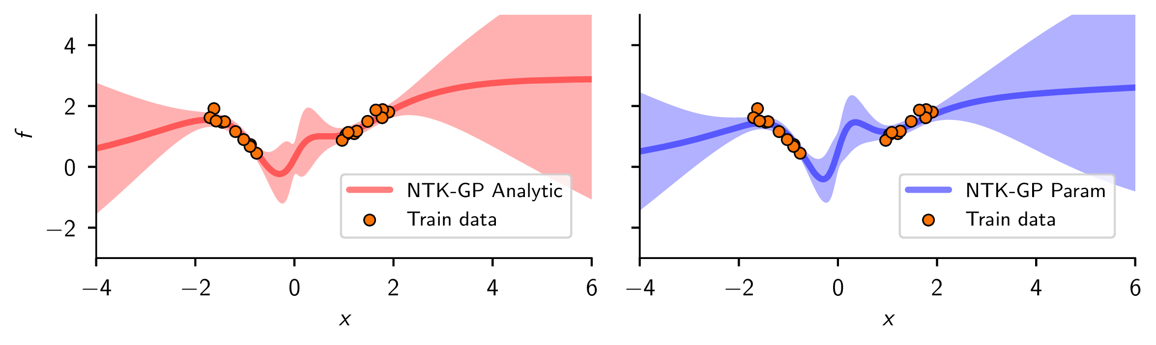
NTK-GP

Using finite width neural networks, we can approximate the Bayesian posterior predictive distribution of a Gaussian process, which closely resembles the true posterior predictive distribution (when available).