Introduction to Variational Inference

Advanced Statistical Inference

Simone Rossi

EURECOM

Introduction to Variational Inference

\[ \require{physics} \definecolor{input}{rgb}{0.42, 0.55, 0.74} \definecolor{params}{rgb}{0.51,0.70,0.40} \definecolor{output}{rgb}{0.843, 0.608, 0} \definecolor{vparams}{rgb}{0.58, 0, 0.83} \definecolor{noise}{rgb}{0.0, 0.48, 0.65} \definecolor{latent}{rgb}{0.8, 0.0, 0.8} \]

Refresher: Kullback-Leibler Divergence

The Kullback-Leibler (KL) divergence is a measure of how one probability distribution diverges from a second
Given two probability distributions \(p({\textcolor{input}{\boldsymbol{x}}})\) and \(q({\textcolor{input}{\boldsymbol{x}}})\), the KL divergence is defined as

\[ \text{KL}\left(q \parallel p\right) = \int q({\textcolor{input}{\boldsymbol{x}}}) \log \frac{q({\textcolor{input}{\boldsymbol{x}}})}{p({\textcolor{input}{\boldsymbol{x}}})} \dd{{\textcolor{input}{\boldsymbol{x}}}} = {\mathbb{E}}_q \left[ \log \frac{q({\textcolor{input}{\boldsymbol{x}}})}{p({\textcolor{input}{\boldsymbol{x}}})} \right] \]

Properties

\(\text{KL}\left(q \parallel p\right) \geq 0\) with equality if and only if \(q({\textcolor{input}{\boldsymbol{x}}}) = p({\textcolor{input}{\boldsymbol{x}}})\)
\(\text{KL}\left(q \parallel p\right) \neq \text{KL}\left(p \parallel q\right)\), i.e., it is not symmetric
It’s not a true distance measure as it’s not symmetric and doesn’t satisfy the triangle inequality

Asymmetry of KL Divergence

KL divergence for Gaussians

The KL divergence between two Gaussians is tractable and has a closed-form solution
For two Gaussian distributions \(p(x) = {\mathcal{N}}(\mu_p, \sigma_p^2)\) and \(q(x) = {\mathcal{N}}(\mu_q, \sigma_q^2)\):

\[ \text{KL}\left(q \parallel p\right) = \frac{1}{2} \left( \frac{\sigma_p^2}{\sigma_q^2} + \frac{(\mu_q - \mu_p)^2}{\sigma_q^2} - 1 + \log \frac{\sigma_p^2}{\sigma_q^2} \right) \]

For two multivariate Gaussians \(p({\textcolor{input}{\boldsymbol{x}}}) = {\mathcal{N}}({\boldsymbol{\mu}}_p, {\boldsymbol{\Sigma}}_p)\) and \(q({\textcolor{input}{\boldsymbol{x}}}) = {\mathcal{N}}({\boldsymbol{\mu}}_q, {\boldsymbol{\Sigma}}_q)\):

\[ \text{KL}\left(q \parallel p\right) = \frac{1}{2} \left( \tr({\boldsymbol{\Sigma}}_q^{-1} {\boldsymbol{\Sigma}}_p) + ({\boldsymbol{\mu}}_q - {\boldsymbol{\mu}}_p)^\top {\boldsymbol{\Sigma}}_q^{-1} ({\boldsymbol{\mu}}_q - {\boldsymbol{\mu}}_p) - k + \log \frac{\det {\boldsymbol{\Sigma}}_q}{\det {\boldsymbol{\Sigma}}_p} \right) \]

Exercise

Simplify the expression when \({\boldsymbol{\Sigma}}_p = \sigma_p^2 {\boldsymbol{I}}\) and \({\boldsymbol{\mu}}_p = {\boldsymbol{0}}\).

Jensen’s Inequality

Another important result is Jensen’s inequality, which states that for any convex function \(f\) and random variable \(X\): \[ {\mathbb{E}}[f(X)] \geq f({\mathbb{E}}[X]) \]

For example, if \(f(x) = \log x\), then:

\[ {\mathbb{E}}[\log X] \leq \log({\mathbb{E}}[X]) \]

Variational Inference

Introduction to Variational Inference

Remember: given a likelihood \(p({\textcolor{output}{\boldsymbol{y}}}\mid {\textcolor{params}{\boldsymbol{\theta}}})\) and a prior \(p({\textcolor{params}{\boldsymbol{\theta}}})\), we want to compute the posterior \(p({\textcolor{params}{\boldsymbol{\theta}}}\mid {\textcolor{output}{\boldsymbol{y}}})\), which is intractable in most cases.

Variational Inference (VI) is a method for approximating intractable posterior distributions

Intuition: Instead of trying to solve intractable integrals, we solve an optimization problem

Sketch of the recipe

Choose a family of distributions \(\mathcal Q\) to approximate the posterior
Define an objective function to measure the quality of the approximation
In the set of distributions \(\mathcal Q\), find the one that minimizes the objective function

[width=80%]

Variational Inference: A Simple Example

Variational Inference: Form of the Approximation

Form of the Approximation

What family of distributions \(q({\textcolor{params}{\boldsymbol{\theta}}})\) should we choose to approximate the posterior \(p({\textcolor{params}{\boldsymbol{\theta}}}\mid {\textcolor{output}{\boldsymbol{y}}})\)?

Mean-field approach: each parameter \(\textcolor{params}\theta_j\) is independent and has its own distribution \[ q({\textcolor{params}{\boldsymbol{\theta}}}) = \prod_{j=1}^J q_j(\textcolor{params}\theta_j) \]

For simplicity:

all \(q_j(\textcolor{params}\theta_j)\) are Gaussian distributions, i.e., \(q_j(\textcolor{params}\theta_j) = q(\textcolor{params}\theta_j) = {\mathcal{N}}(\textcolor{vparams}m_j, \textcolor{vparams}s_j^2)\)
each parameter \(\textcolor{params}\theta_j\) has its own mean \(\textcolor{vparams}m_j\) and variance \(\textcolor{vparams}s_j^2\)

\[ q({\textcolor{params}{\boldsymbol{\theta}}}) = \prod_{j=1}^J {\mathcal{N}}(\textcolor{vparams}\mu_j, \textcolor{vparams}\sigma_j^2) \]

\({\textcolor{vparams}{\boldsymbol{\nu}}}= \{\textcolor{vparams}m_j, \textcolor{vparams}s_j^2\}\) are called the variational parameters
The goal is to find the optimal values of \({\textcolor{vparams}{\boldsymbol{\nu}}}\) \(\Rightarrow\) best approximation \(q({\textcolor{params}{\boldsymbol{\theta}}};{\textcolor{vparams}{\boldsymbol{\nu}}})\) to the true posterior

Defining the Objective Function

Objective Function

How to define the quality of the approximation \(q({\textcolor{params}{\boldsymbol{\theta}}};{\textcolor{vparams}{\boldsymbol{\nu}}})\)?

We use the KL divergence between the approximate distribution \(q({\textcolor{params}{\boldsymbol{\theta}}};{\textcolor{vparams}{\boldsymbol{\nu}}})\) and the true posterior \(p({\textcolor{params}{\boldsymbol{\theta}}}\mid {\textcolor{output}{\boldsymbol{y}}})\)

Problem

This expression is still intractable because the posterior \(p({\textcolor{params}{\boldsymbol{\theta}}}\mid {\textcolor{output}{\boldsymbol{y}}})\) is unknown
We need to find a way to approximate the KL divergence

Manipluating the expression:

\[ \begin{aligned} \text{KL}\left(q({\textcolor{params}{\boldsymbol{\theta}}};{\textcolor{vparams}{\boldsymbol{\nu}}}) \parallel p({\textcolor{params}{\boldsymbol{\theta}}}\mid {\textcolor{output}{\boldsymbol{y}}})\right) &= {\mathbb{E}}_{q({\textcolor{params}{\boldsymbol{\theta}}};{\textcolor{vparams}{\boldsymbol{\nu}}})} \log q({\textcolor{params}{\boldsymbol{\theta}}};{\textcolor{vparams}{\boldsymbol{\nu}}}) - {\mathbb{E}}_{q({\textcolor{params}{\boldsymbol{\theta}}};{\textcolor{vparams}{\boldsymbol{\nu}}})} \log p({\textcolor{params}{\boldsymbol{\theta}}}\mid {\textcolor{output}{\boldsymbol{y}}}) \\ &= {\mathbb{E}}_{q({\textcolor{params}{\boldsymbol{\theta}}};{\textcolor{vparams}{\boldsymbol{\nu}}})} \log q({\textcolor{params}{\boldsymbol{\theta}}};{\textcolor{vparams}{\boldsymbol{\nu}}}) - {\mathbb{E}}_{q({\textcolor{params}{\boldsymbol{\theta}}};{\textcolor{vparams}{\boldsymbol{\nu}}})} \log \frac{p({\textcolor{output}{\boldsymbol{y}}}\mid{\textcolor{params}{\boldsymbol{\theta}}})p({\textcolor{params}{\boldsymbol{\theta}}})}{p({\textcolor{output}{\boldsymbol{y}}})} \\ &= \underbrace{{\mathbb{E}}_{q({\textcolor{params}{\boldsymbol{\theta}}};{\textcolor{vparams}{\boldsymbol{\nu}}})} \log q({\textcolor{params}{\boldsymbol{\theta}}};{\textcolor{vparams}{\boldsymbol{\nu}}})}_{\bigcirc\llap{\text{\small 1}\kern .3em}} - \underbrace{{\mathbb{E}}_{q({\textcolor{params}{\boldsymbol{\theta}}};{\textcolor{vparams}{\boldsymbol{\nu}}})} \log p({\textcolor{output}{\boldsymbol{y}}}\mid{\textcolor{params}{\boldsymbol{\theta}}})}_{\bigcirc\llap{\text{\small 2}\kern .3em}} - \underbrace{{\mathbb{E}}_{q({\textcolor{params}{\boldsymbol{\theta}}};{\textcolor{vparams}{\boldsymbol{\nu}}})} \log p({\textcolor{params}{\boldsymbol{\theta}}})}_{\bigcirc\llap{\text{\small 3}\kern .3em}} + \underbrace{\log p({\textcolor{output}{\boldsymbol{y}}})}_{\bigcirc\llap{\text{\small 4}\kern .3em}} \end{aligned} \]

Breakdown:

\(\bigcirc\llap{\text{\small 1}\kern .3em}\): entropy of the variational distribution \(q({\textcolor{params}{\boldsymbol{\theta}}};{\textcolor{vparams}{\boldsymbol{\nu}}})\)

\(\bigcirc\llap{\text{\small 2}\kern .3em}\): expected log-likelihood of the data under the variational distribution

\(\bigcirc\llap{\text{\small 3}\kern .3em}\): cross-entropy between the variational distribution and the prior

\(\bigcirc\llap{\text{\small 4}\kern .3em}\): log marginal likelihood of the data

Rearranging the terms:

This is an important equation in variational inference!

Note: The term \(\log p({\textcolor{output}{\boldsymbol{y}}})\) is a constant w.r.t. \({\textcolor{vparams}{\boldsymbol{\nu}}}\). Let’s move it to the left:

\[ \begin{aligned} \log p({\textcolor{output}{\boldsymbol{y}}}) - \text{KL}\left(q({\textcolor{params}{\boldsymbol{\theta}}};{\textcolor{vparams}{\boldsymbol{\nu}}}) \parallel p({\textcolor{params}{\boldsymbol{\theta}}}\mid {\textcolor{output}{\boldsymbol{y}}})\right) &= {\mathbb{E}}_{q({\textcolor{params}{\boldsymbol{\theta}}};{\textcolor{vparams}{\boldsymbol{\nu}}})} \log p({\textcolor{output}{\boldsymbol{y}}}\mid{\textcolor{params}{\boldsymbol{\theta}}}) - \text{KL}\left(q({\textcolor{params}{\boldsymbol{\theta}}};{\textcolor{vparams}{\boldsymbol{\nu}}}) \parallel p({\textcolor{params}{\boldsymbol{\theta}}})\right) \end{aligned} \]

Now the right-hand side is computable: it’s called Evidence Lower Bound (ELBO)

\[ {\mathcal{L}}_{\text{ELBO}}({\textcolor{vparams}{\boldsymbol{\nu}}}) = {\mathbb{E}}_{q({\textcolor{params}{\boldsymbol{\theta}}};{\textcolor{vparams}{\boldsymbol{\nu}}})} \log p({\textcolor{output}{\boldsymbol{y}}}\mid{\textcolor{params}{\boldsymbol{\theta}}}) - \text{KL}\left(q({\textcolor{params}{\boldsymbol{\theta}}};{\textcolor{vparams}{\boldsymbol{\nu}}}) \parallel p({\textcolor{params}{\boldsymbol{\theta}}})\right) \]

ELBO: Evidence Lower Bound

\[ \log p({\textcolor{output}{\boldsymbol{y}}}) - \text{KL}\left(q({\textcolor{params}{\boldsymbol{\theta}}};{\textcolor{vparams}{\boldsymbol{\nu}}}) \parallel p({\textcolor{params}{\boldsymbol{\theta}}}\mid {\textcolor{output}{\boldsymbol{y}}})\right) = {\mathcal{L}}_{\text{ELBO}}({\textcolor{vparams}{\boldsymbol{\nu}}}) \]

Minimizing the KL divergence is equivalent to maximizing the ELBO
The KL divergence is non-negative:
1. \({\mathcal{L}}_{\text{ELBO}}({\textcolor{vparams}{\boldsymbol{\nu}}}) \leq \log p({\textcolor{output}{\boldsymbol{y}}})\)
2. \({\mathcal{L}}_{\text{ELBO}}({\textcolor{vparams}{\boldsymbol{\nu}}})\) is a lower bound on the marginal likelihood of the data
3. If \(q({\textcolor{params}{\boldsymbol{\theta}}};{\textcolor{vparams}{\boldsymbol{\nu}}}) = p({\textcolor{params}{\boldsymbol{\theta}}}\mid {\textcolor{output}{\boldsymbol{y}}})\), then \({\mathcal{L}}_{\text{ELBO}}({\textcolor{vparams}{\boldsymbol{\nu}}}) = \log p({\textcolor{output}{\boldsymbol{y}}})\)

ELBO to be maximized w.r.t. the variational parameters \({\textcolor{vparams}{\boldsymbol{\nu}}}\):

\[ \begin{aligned} {\mathcal{L}}_{\text{ELBO}}({\textcolor{vparams}{\boldsymbol{\nu}}}) &= {\mathbb{E}}_{q({\textcolor{params}{\boldsymbol{\theta}}};{\textcolor{vparams}{\boldsymbol{\nu}}})} \log p({\textcolor{output}{\boldsymbol{y}}}\mid{\textcolor{params}{\boldsymbol{\theta}}}) - \text{KL}\left(q({\textcolor{params}{\boldsymbol{\theta}}};{\textcolor{vparams}{\boldsymbol{\nu}}}) \parallel p({\textcolor{params}{\boldsymbol{\theta}}})\right) \end{aligned} \]

The first term is a model fitting term:
- It encourages the model to explain the data well
- The higher, the better the parameters drawn from \(q({\textcolor{params}{\boldsymbol{\theta}}};{\textcolor{vparams}{\boldsymbol{\nu}}})\) are at explaining the data
The second term is a regularization term:
- It encourages the variational distribution to be close to the prior
- The lower, the closer the variational distribution is to the prior

Computing the ELBO: Regularization Term

Recall our assumption that the variational distribution is a product of Gaussians \(q({\textcolor{params}{\boldsymbol{\theta}}}) = \prod_{j=1}^J {\mathcal{N}}(\textcolor{vparams}m_j, \textcolor{vparams}s_j^2)\)
The second term in the ELBO is the KL divergence between the variational distribution and the prior \(p({\textcolor{params}{\boldsymbol{\theta}}}) = \prod_{j=1}^J {\mathcal{N}}(0, \sigma^2)\)
The KL divergence between two Gaussians is tractable and has a closed-form solution

\[ \begin{aligned} \text{KL}\left(q({\textcolor{params}{\boldsymbol{\theta}}};{\textcolor{vparams}{\boldsymbol{\nu}}}) \parallel p({\textcolor{params}{\boldsymbol{\theta}}})\right) &= \frac 1 2 \sum_{j=1}^J \left( \frac{\textcolor{vparams}s_j^2}{\sigma^2} + \frac{\textcolor{vparams}m_j^2}{\sigma^2} - 1 + \log \frac{\sigma^2}{\textcolor{vparams}s_j^2} \right) \end{aligned} \]

Computing the ELBO: Model Fitting Term

The first term is more complex to compute and only analytically available for simple models, but …

… we can use Monte Carlo methods to estimate it

\[ \begin{aligned} {\mathbb{E}}_{q({\textcolor{params}{\boldsymbol{\theta}}};{\textcolor{vparams}{\boldsymbol{\nu}}})} \log p({\textcolor{output}{\boldsymbol{y}}}\mid{\textcolor{params}{\boldsymbol{\theta}}}) &\approx \frac 1 S \sum_{s=1}^S \log p({\textcolor{output}{\boldsymbol{y}}}\mid{\textcolor{params}{\boldsymbol{\theta}}}^{(s)}) \end{aligned} \]

where \({\textcolor{params}{\boldsymbol{\theta}}}^{(s)} \sim q({\textcolor{params}{\boldsymbol{\theta}}};{\textcolor{vparams}{\boldsymbol{\nu}}})\)

Note: This estimation is unbiased and its variance decreases with \(\propto 1/S\), independent of the dimensionality of \({\textcolor{params}{\boldsymbol{\theta}}}\)!

ELBO Optimization

Review:

We chose a family of distributions \(\mathcal Q\) to approximate the posterior (\(q({\textcolor{params}{\boldsymbol{\theta}}};{\textcolor{vparams}{\boldsymbol{\nu}}}) = \prod_{j=1}^J {\mathcal{N}}(\textcolor{vparams}m_j, \textcolor{vparams}s_j^2)\))
We defined the ELBO as the objective function to measure the quality of the approximation \[ {\mathcal{L}}_{\text{ELBO}}({\textcolor{vparams}{\boldsymbol{\nu}}}) = {\mathbb{E}}_{q({\textcolor{params}{\boldsymbol{\theta}}};{\textcolor{vparams}{\boldsymbol{\nu}}})} \log p({\textcolor{output}{\boldsymbol{y}}}\mid{\textcolor{params}{\boldsymbol{\theta}}}) - \text{KL}\left(q({\textcolor{params}{\boldsymbol{\theta}}};{\textcolor{vparams}{\boldsymbol{\nu}}}) \parallel p({\textcolor{params}{\boldsymbol{\theta}}})\right) \]
We discussed how to compute the regularization term and the model fitting term

We need to optimize the ELBO w.r.t. the variational parameters \({\textcolor{vparams}{\boldsymbol{\nu}}}\)

\[ \begin{aligned} {\textcolor{vparams}{\boldsymbol{\nu}}}^* &= \arg\max_{{\textcolor{vparams}{\boldsymbol{\nu}}}} {\mathcal{L}}_{\text{ELBO}}({\textcolor{vparams}{\boldsymbol{\nu}}}) \\ &= \arg\max_{{\textcolor{vparams}{\boldsymbol{\nu}}}} {\mathbb{E}}_{q({\textcolor{params}{\boldsymbol{\theta}}};{\textcolor{vparams}{\boldsymbol{\nu}}})} \log p({\textcolor{output}{\boldsymbol{y}}}\mid{\textcolor{params}{\boldsymbol{\theta}}}) - \text{KL}\left(q({\textcolor{params}{\boldsymbol{\theta}}};{\textcolor{vparams}{\boldsymbol{\nu}}}) \parallel p({\textcolor{params}{\boldsymbol{\theta}}})\right) \end{aligned} \]

An overview of VI optimization algorithms

VI algorithms can be divided into two categories:

Coordinate Ascent Variational Inference (CAVI):
- Optimize each variational parameter \(\textcolor{vparams}\nu_j\) separately
Gradient-based Variational Inference:
- Use gradient-based optimization methods to optimize the variational parameters simultaneously

Gradient-based methods comes in different flavors:

Black-box Variational Inference (BBVI)
Reparameterization Gradients (RG)
Stochastic Variational Inference (SVI)
Automatic Differentiation Variational Inference (ADVI)
Amortized Variational Inference

Optimizing the ELBO is hard

Let’s consider the optimization problem:

We need to compute the gradient of the ELBO w.r.t. the variational parameters \({\textcolor{vparams}{\boldsymbol{\nu}}}\):

\[ \begin{aligned} \grad_{{\textcolor{vparams}{\boldsymbol{\nu}}}} {\mathcal{L}}_{\text{ELBO}}({\textcolor{vparams}{\boldsymbol{\nu}}}) &= \grad_{{\textcolor{vparams}{\boldsymbol{\nu}}}} {\mathbb{E}}_{q({\textcolor{params}{\boldsymbol{\theta}}};{\textcolor{vparams}{\boldsymbol{\nu}}})} \log p({\textcolor{output}{\boldsymbol{y}}}\mid{\textcolor{params}{\boldsymbol{\theta}}}) - \grad_{{\textcolor{vparams}{\boldsymbol{\nu}}}} \text{KL}\left(q({\textcolor{params}{\boldsymbol{\theta}}};{\textcolor{vparams}{\boldsymbol{\nu}}}) \parallel p({\textcolor{params}{\boldsymbol{\theta}}})\right) \end{aligned} \]

Problem

We cannot move the gradient inside the expectation because the expectation is w.r.t. the variational distribution \(q({\textcolor{params}{\boldsymbol{\theta}}};{\textcolor{vparams}{\boldsymbol{\nu}}})\)

REINFORCE: The Score Function Gradient Estimator

The Score Function Gradient Estimator (REINFORCE) is a general method to estimate gradients of expectations

Log-derivative trick:

\[ \begin{aligned} \grad_{{\textcolor{vparams}{\boldsymbol{\nu}}}} q({\textcolor{params}{\boldsymbol{\theta}}};{\textcolor{vparams}{\boldsymbol{\nu}}}) &= q({\textcolor{params}{\boldsymbol{\theta}}};{\textcolor{vparams}{\boldsymbol{\nu}}}) \grad_{{\textcolor{vparams}{\boldsymbol{\nu}}}} \log q({\textcolor{params}{\boldsymbol{\theta}}};{\textcolor{vparams}{\boldsymbol{\nu}}}) \end{aligned} \]

Derivation

Derive the expression above using the chain rule

\[ \begin{aligned} \grad_{{\boldsymbol{z}}} \log f({\boldsymbol{z}}) &= \frac{\grad_{{\boldsymbol{z}}} f({\boldsymbol{z}})}{f({\boldsymbol{z}})} \end{aligned} \]

Then, rearrange the terms

REINFORCE: The Score Function Gradient Estimator

Using the log-derivative trick, we can rewrite the gradient of the ELBO w.r.t. the variational parameters \({\textcolor{vparams}{\boldsymbol{\nu}}}\):

where \({\textcolor{params}{\boldsymbol{\theta}}}^{(s)} \sim q({\textcolor{params}{\boldsymbol{\theta}}};{\textcolor{vparams}{\boldsymbol{\nu}}})\).

REINFORCE: The Score Function Gradient Estimator

Pros

Easy to implement
Only requires the gradient of the log-density of the variational distribution
Can be used for any model (hence the name “black-box”)

Cons

High variance
Slow convergence
Needs additional variance reduction techniques
Not popular for (modern) variational inference

Reparameterization Trick

Objective: \(\grad_{{\textcolor{vparams}{\boldsymbol{\nu}}}} {\mathbb{E}}_{q({\textcolor{params}{\boldsymbol{\theta}}};{\textcolor{vparams}{\boldsymbol{\nu}}})} \log p({\textcolor{output}{\boldsymbol{y}}}\mid{\textcolor{params}{\boldsymbol{\theta}}})\)

Idea: Freeze the randomness in the variational distribution

Samples from \(q({\textcolor{params}{\boldsymbol{\theta}}};{\textcolor{vparams}{\boldsymbol{\nu}}})\) are generated by a deterministic transformation \(t\) of a random variable \({\textcolor{noise}{\boldsymbol{\varepsilon}}}\sim p({\textcolor{noise}{\boldsymbol{\varepsilon}}})\)
The variational parameters \({\textcolor{vparams}{\boldsymbol{\nu}}}\) are parameters of the transformation \(t\)
The gradient of the expectation w.r.t. the variational parameters can be computed using the chain rule

Gaussian Example

For a Gaussian variational distribution \(q({\textcolor{params}{\boldsymbol{\theta}}}_i;{\textcolor{vparams}{\boldsymbol{\nu}}}) = {\mathcal{N}}(\textcolor{vparams}m_i, \textcolor{vparams}s_i^2)\)

\(p({\textcolor{noise}{\boldsymbol{\varepsilon}}}) = {\mathcal{N}}(0, 1)\)
\(t({\textcolor{noise}{\boldsymbol{\varepsilon}}}; {\textcolor{vparams}{\boldsymbol{\nu}}}) = \textcolor{vparams}m_i + \textcolor{vparams}s_i {\textcolor{noise}{\boldsymbol{\varepsilon}}}\)

Reparameterization Trick: Derivation

Key observation

For a generic function \(f({\textcolor{params}{\boldsymbol{\theta}}})\), we have \[ \begin{aligned} \grad_{{\textcolor{vparams}{\boldsymbol{\nu}}}} {\mathbb{E}}_{q({\textcolor{params}{\boldsymbol{\theta}}};{\textcolor{vparams}{\boldsymbol{\nu}}})} f({\textcolor{params}{\boldsymbol{\theta}}}) &= \grad_{{\textcolor{vparams}{\boldsymbol{\nu}}}} {\mathbb{E}}_{p({\textcolor{noise}{\boldsymbol{\varepsilon}}})} f({\textcolor{params}{\boldsymbol{\theta}}}) \end{aligned} \]

with \({\textcolor{params}{\boldsymbol{\theta}}}= t({\textcolor{noise}{\boldsymbol{\varepsilon}}}; {\textcolor{vparams}{\boldsymbol{\nu}}})\). Now the expectation is w.r.t. the random variable \({\textcolor{noise}{\boldsymbol{\varepsilon}}}\) and the gradient can be moved inside the expectation

For the ELBO:

\[ \begin{aligned} \grad_{{\textcolor{vparams}{\boldsymbol{\nu}}}} {\mathbb{E}}_{q({\textcolor{params}{\boldsymbol{\theta}}};{\textcolor{vparams}{\boldsymbol{\nu}}})} \log p({\textcolor{output}{\boldsymbol{y}}}\mid{\textcolor{params}{\boldsymbol{\theta}}}) &= \grad_{{\textcolor{vparams}{\boldsymbol{\nu}}}} {\mathbb{E}}_{p({\textcolor{noise}{\boldsymbol{\varepsilon}}})} \log p({\textcolor{output}{\boldsymbol{y}}}\mid {\textcolor{params}{\boldsymbol{\theta}}}) \\ &\class{fragment}{{} = {\mathbb{E}}_{p({\textcolor{noise}{\boldsymbol{\varepsilon}}})} \grad_{{\textcolor{vparams}{\boldsymbol{\nu}}}} \log p({\textcolor{output}{\boldsymbol{y}}}\mid {\textcolor{params}{\boldsymbol{\theta}}})} \\ &\class{fragment}{{} = {\mathbb{E}}_{p({\textcolor{noise}{\boldsymbol{\varepsilon}}})} \grad_{{\textcolor{params}{\boldsymbol{\theta}}}} \log p({\textcolor{output}{\boldsymbol{y}}}\mid {\textcolor{params}{\boldsymbol{\theta}}}) \grad_{{\textcolor{vparams}{\boldsymbol{\nu}}}} {\textcolor{params}{\boldsymbol{\theta}}}} \\ &\class{fragment}{{} = {\mathbb{E}}_{p({\textcolor{noise}{\boldsymbol{\varepsilon}}})} \grad_{{\textcolor{params}{\boldsymbol{\theta}}}} \log p({\textcolor{output}{\boldsymbol{y}}}\mid {\textcolor{params}{\boldsymbol{\theta}}}) \grad_{{\textcolor{vparams}{\boldsymbol{\nu}}}} t({\textcolor{noise}{\boldsymbol{\varepsilon}}}; {\textcolor{vparams}{\boldsymbol{\nu}}})} \\ &\class{fragment}{{} \approx \frac 1 S \sum_{s=1}^S \grad_{{\textcolor{params}{\boldsymbol{\theta}}}} \log p({\textcolor{output}{\boldsymbol{y}}}\mid {\textcolor{params}{\boldsymbol{\theta}}}^{(s)}) \grad_{{\textcolor{vparams}{\boldsymbol{\nu}}}} t({\textcolor{noise}{\boldsymbol{\varepsilon}}}^{(s)}; {\textcolor{vparams}{\boldsymbol{\nu}}})} \end{aligned} \]

where \({\textcolor{noise}{\boldsymbol{\varepsilon}}}^{(s)} \sim p({\textcolor{noise}{\boldsymbol{\varepsilon}}})\) and \({\textcolor{params}{\boldsymbol{\theta}}}^{(s)} = t({\textcolor{noise}{\boldsymbol{\varepsilon}}}^{(s)}; {\textcolor{vparams}{\boldsymbol{\nu}}})\).

Reparameterization Trick: Pros and Cons

Pros

Low variance
Fast convergence
No need for additional variance reduction techniques
Popular in many models (like autoencoders)

Cons

Requires reparameterization of the variational distribution
Needs the model/likelihood to be differentiable

Reparameterization Gradients vs REINFORCE

Comparison of the gradients of the ELBO w.r.t. the variational parameters using the Reparameterization Gradients and REINFORCE

Stochastic Gradient Optimization

The gradient of the ELBO w.r.t. the variational parameters \({\textcolor{vparams}{\boldsymbol{\nu}}}\) are stochastic but unbiased

\[ {\mathbb{E}}_{\text{noise}} \widetilde{\grad_{{\textcolor{vparams}{\boldsymbol{\nu}}}} {\mathcal{L}}_{\text{ELBO}}({\textcolor{vparams}{\boldsymbol{\nu}}})} = \grad_{{\textcolor{vparams}{\boldsymbol{\nu}}}} {\mathcal{L}}_{\text{ELBO}}({\textcolor{vparams}{\boldsymbol{\nu}}}) \]

Variational inference with stochastic optimization

Stochastic optimization has a long history and good theoretical properties about convergence
Optimizing using stochastic updates reaches local optima if the learning rate \(\alpha_t\) goes to zero with a certain rate (Robbins-Monro conditions)

\[ \begin{aligned} \sum_i^T \alpha_i = \infty \quad \text{and} \quad \sum_i^T \alpha_i^2 < \infty \end{aligned} \]

Price: Covergence in \(\mathcal{O}(1/\sqrt{T})\) where \(T\) is the number of iterations, vs \(\mathcal{O}(1/T)\) with exact gradients (when available)

Convergence of Stochastic Optimization

\[ \begin{aligned} {\textcolor{vparams}{\boldsymbol{\nu}}}_{t+1} &= {\textcolor{vparams}{\boldsymbol{\nu}}}_t + \alpha_t \widetilde{\grad_{{\textcolor{vparams}{\boldsymbol{\nu}}}} {\mathcal{L}}_{\text{ELBO}}({\textcolor{vparams}{\boldsymbol{\nu}}}_t)} \end{aligned} \]

Summary

Variational Inference (VI) is a method for approximating intractable posterior distributions
The goal is to find the best approximation \(q({\textcolor{params}{\boldsymbol{\theta}}};{\textcolor{vparams}{\boldsymbol{\nu}}})\) to the true posterior \(p({\textcolor{params}{\boldsymbol{\theta}}}\mid {\textcolor{output}{\boldsymbol{y}}})\)
The quality of the approximation is measured using the Evidence Lower Bound (ELBO)
Optimizing the ELBO w.r.t. the variational parameters \({\textcolor{vparams}{\boldsymbol{\nu}}}\) is challenging:
The gradients of the ELBO are generally intractable
We can use Monte Carlo methods to estimate the gradient

Extensions

Extensions of Variational Inference

Mini-batch optimization
More complex variational families

Mini-batch Optimization

Likelihood term in the ELBO: \({\mathbb{E}}_{q({\textcolor{params}{\boldsymbol{\theta}}};{\textcolor{vparams}{\boldsymbol{\nu}}})} \log p({\textcolor{output}{\boldsymbol{y}}}\mid{\textcolor{params}{\boldsymbol{\theta}}})\)
If the likelihood factorizes over the data points (data points are independent):

\[ \begin{aligned} {\mathbb{E}}_{q({\textcolor{params}{\boldsymbol{\theta}}};{\textcolor{vparams}{\boldsymbol{\nu}}})} \log p({\textcolor{output}{\boldsymbol{y}}}\mid{\textcolor{params}{\boldsymbol{\theta}}}) &= \sum_{i=1}^N {\mathbb{E}}_{q({\textcolor{params}{\boldsymbol{\theta}}};{\textcolor{vparams}{\boldsymbol{\nu}}})} \log p({\textcolor{output}{\boldsymbol{y}}}_i\mid{\textcolor{params}{\boldsymbol{\theta}}}) \end{aligned} \]

Problem:

We need to compute the expectation over the variational distribution for each data point
For large datasets, this can be computationally expensive

Solution: Use mini-batches of data points to estimate the expectation

\[ \begin{aligned} {\mathbb{E}}_{q({\textcolor{params}{\boldsymbol{\theta}}};{\textcolor{vparams}{\boldsymbol{\nu}}})} \log p({\textcolor{output}{\boldsymbol{y}}}\mid{\textcolor{params}{\boldsymbol{\theta}}}) &\approx \frac N B \sum_{b=1}^B {\mathbb{E}}_{q({\textcolor{params}{\boldsymbol{\theta}}};{\textcolor{vparams}{\boldsymbol{\nu}}})} \log p({\textcolor{output}{\boldsymbol{y}}}_i\mid{\textcolor{params}{\boldsymbol{\theta}}}) \quad \text{with} \quad B \ll N \end{aligned} \]

Mini-batch Optimization

\[ \begin{aligned} {\mathbb{E}}_{q({\textcolor{params}{\boldsymbol{\theta}}};{\textcolor{vparams}{\boldsymbol{\nu}}})} \log p({\textcolor{output}{\boldsymbol{y}}}\mid{\textcolor{params}{\boldsymbol{\theta}}}) &\approx \frac N B \sum_{b=1}^B {\mathbb{E}}_{q({\textcolor{params}{\boldsymbol{\theta}}};{\textcolor{vparams}{\boldsymbol{\nu}}})} \log p({\textcolor{output}{\boldsymbol{y}}}_i\mid{\textcolor{params}{\boldsymbol{\theta}}}) \end{aligned} \]

Pros: - Faster convergence - Scalable to large datasets

But double source of stochasticity:

Monte Carlo estimation of the expectation
Mini-batch optimization

More Complex Variational Families

Mean-field assumption: each parameter \(\textcolor{params}\theta_j\) is independent and has its own distribution
Problem: The mean-field assumption can be too restrictive \(\Rightarrow\) we can use more complex variational families
If we make the variational family more complex, we get better approximation to the true posterior

Gaussian with Full Covariance

Instead of assuming that the parameters are independent, we can assume that they are correlated

The variational distribution is a multivariate Gaussian with full covariance matrix

\[ \begin{aligned} q({\textcolor{params}{\boldsymbol{\theta}}}) &= {\mathcal{N}}(\textcolor{vparams}{\boldsymbol{\mu}}, \textcolor{vparams}{\boldsymbol{\Sigma}}) \end{aligned} \]

Reparameterization trick is still applicable using the Cholesky decomposition \(\textcolor{vparams}{\boldsymbol{\Sigma}}= \textcolor{vparams}{\boldsymbol{L}}\textcolor{vparams}{\boldsymbol{L}}^T\)

\[ \begin{aligned} {\textcolor{params}{\boldsymbol{\theta}}}&= \textcolor{vparams}{\boldsymbol{\mu}}+ \textcolor{vparams}{\boldsymbol{L}}{\textcolor{noise}{\boldsymbol{\varepsilon}}}, \quad \text{with} \quad {\textcolor{noise}{\boldsymbol{\varepsilon}}}\sim {\mathcal{N}}({\boldsymbol{0}}, {\boldsymbol{I}}) \end{aligned} \]

Example: Gaussian with Full Covariance

Normalizing Flows

Refresh

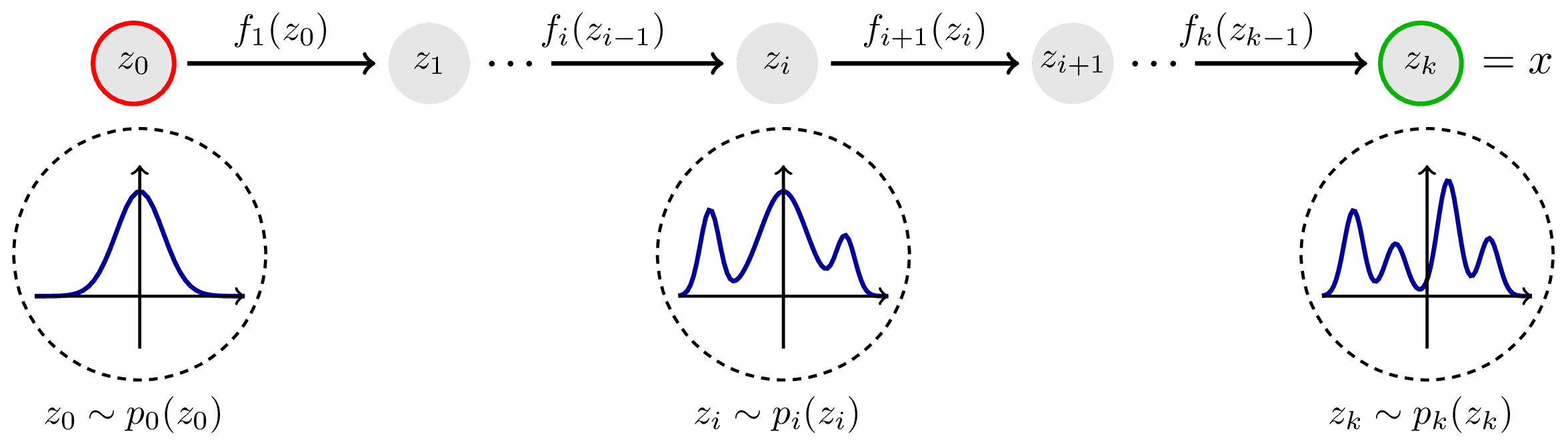
Given a invertible function \(f: \mathcal{X} \mapsto \mathcal{Y}\) and a simple distribution \(p({\textcolor{input}{\boldsymbol{x}}})\), we can compute the density of \({\textcolor{output}{\boldsymbol{y}}}\) as

\[ \begin{aligned} p({\textcolor{output}{\boldsymbol{y}}}) &= p({\textcolor{input}{\boldsymbol{x}}}) \left| \det \left( \frac{\partial f^{-1}}{\partial {\textcolor{output}{\boldsymbol{y}}}} \right) \right| \end{aligned} \]

We need to build \(f\):

complex enough to approximate the true posterior
simple enough to be able to compute the determinant of the Jacobian

Idea: Transform a simple distribution into a complex one using a sequence of invertible transformations

Normalizing Flows

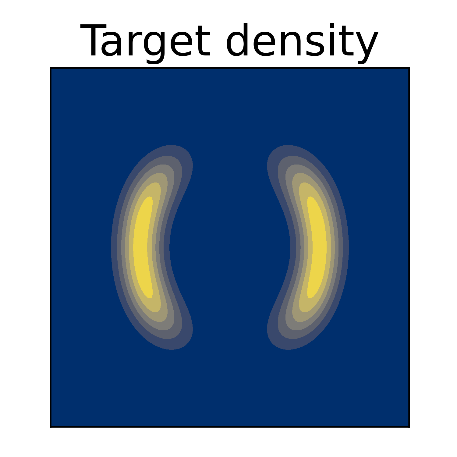
Normalizing Flows: Example

Applications

Applications of Variational Inference

Variational inference is used as inference method in many models:

Latent Dirichlet Allocation (LDA):
- Topic modeling
- Discovering topics in a collection of documents

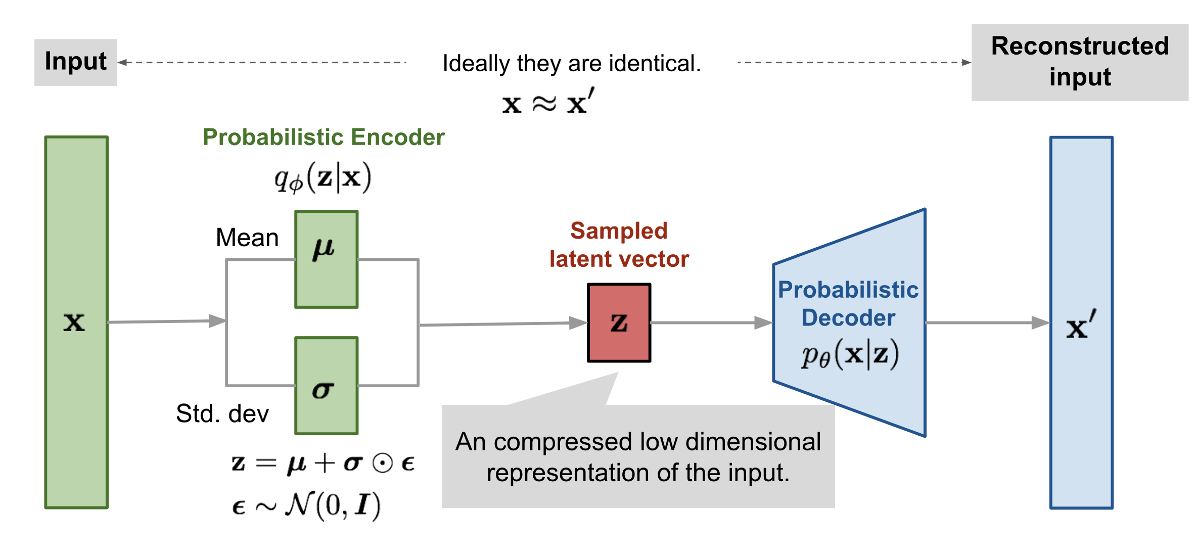
Variational Autoencoders (VAE):
- Generative models
- Learning representations of data