Gaussian Processes
Advanced Statistical Inference
EURECOM
\[ \require{physics} \definecolor{input}{rgb}{0.42, 0.55, 0.74} \definecolor{params}{rgb}{0.51,0.70,0.40} \definecolor{output}{rgb}{0.843, 0.608, 0} \definecolor{vparams}{rgb}{0.58, 0, 0.83} \definecolor{noise}{rgb}{0.0, 0.48, 0.65} \definecolor{latent}{rgb}{0.8, 0.0, 0.8} \definecolor{function}{rgb}{0.75, 0.75, 0.12} \]
Where are we?
We have seen:
- Bayesian linear regression
- Approximate inference
- Markov chain Monte Carlo
- Variational inference
- Laplace approximation
- Bayesian logistic regression (for classification)
- Today: Gaussian processes
Introduction
Gaussian processes (GPs) are a flexible and powerful tool for regression (and classification).
Linear models require us to specify a set of basis functions and their coefficients.
- Polynomials? Trigonometric functions? etc?
Can we use Bayesian inference to let the data decide?
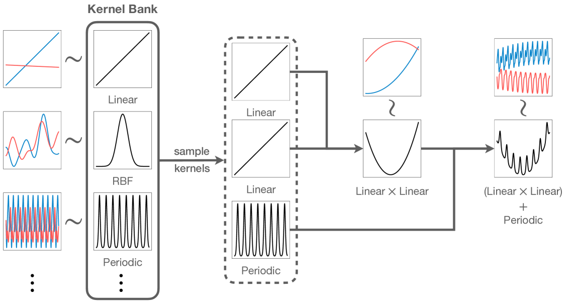
Gaussian processes work implicitly with an infinite-dimensional set of basis functions and learn a probabilistic combination of them.
Gaussian Processes (GPs)
Gaussian processes can be explained in two ways:
- Weight-space view:
- Understand GPs as a Bayesian linear regression model with implicit basis functions.
- Since the basis functions are implicit, we can even work with infinite-dimensional feature spaces.
- Function-space view:
- Understand GPs as a distribution over functions.
- There are no parameters in this view, only functions, so we can implicitly work with infinite-dimensional parameter spaces.
Function-space view of Gaussian Processes
\[ p({\textcolor{input}{\boldsymbol{x}}}) = \mathcal{N}({\textcolor{input}{\boldsymbol{x}}}; {\boldsymbol{\mu}}, {\boldsymbol{\Sigma}}) = \frac{1}{(2 \pi)^{D/2} |{\boldsymbol{\Sigma}}|^{1/2}} \exp \left( -\frac{1}{2} ({\textcolor{input}{\boldsymbol{x}}}- {\boldsymbol{\mu}})^\top {\boldsymbol{\Sigma}}^{-1} ({\textcolor{input}{\boldsymbol{x}}}- {\boldsymbol{\mu}}) \right) \]
Why use Gaussian?
Gaussian distribution have several nice properties that make them attractive:
- Sums of Gaussians are Gaussian.
- Marginals of multivariate Gaussians are Gaussian.
- Conditionals of Gaussians are Gaussian.
Conditioning a Gaussian distribution
\[ {\textcolor{latent}{\boldsymbol{f}}}= \begin{bmatrix} {\textcolor{latent}{\boldsymbol{f}}}_1 \\ {\textcolor{latent}{\boldsymbol{f}}}_2 \end{bmatrix} \sim {\mathcal{N}}\left(\begin{bmatrix} {\boldsymbol{\mu}}_1 \\ {\boldsymbol{\mu}}_2 \end{bmatrix}, \begin{bmatrix} {\boldsymbol{\Sigma}}_{11} & {\boldsymbol{\Sigma}}_{12} \\ {\boldsymbol{\Sigma}}_{21} & {\boldsymbol{\Sigma}}_{22} \end{bmatrix}\right) \]
Then
\[ p({\textcolor{latent}{\boldsymbol{f}}}_2\mid{\textcolor{latent}{\boldsymbol{f}}}_1) = {\mathcal{N}}({\boldsymbol{\mu}}_2 + {\boldsymbol{\Sigma}}_{21}{\boldsymbol{\Sigma}}_{11}^{-1}({\textcolor{latent}{\boldsymbol{f}}}_1 - {\boldsymbol{\mu}}_1), {\boldsymbol{\Sigma}}_{22} - {\boldsymbol{\Sigma}}_{21}{\boldsymbol{\Sigma}}_{11}^{-1}{\boldsymbol{\Sigma}}_{12}) \]
which simplifies if \({\boldsymbol{\mu}}_1, {\boldsymbol{\mu}}_2 = {\boldsymbol{0}}\),
\[ p({\textcolor{latent}{\boldsymbol{f}}}_2\mid{\textcolor{latent}{\boldsymbol{f}}}_1) = {\mathcal{N}}({\boldsymbol{\Sigma}}_{21}{\boldsymbol{\Sigma}}_{11}^{-1}{\textcolor{latent}{\boldsymbol{f}}}_1, {\boldsymbol{\Sigma}}_{22} - {\boldsymbol{\Sigma}}_{21}{\boldsymbol{\Sigma}}_{11}^{-1}{\boldsymbol{\Sigma}}_{12}) \]
Tip
This is sometimes referred to as the Bayes’ rule for Gaussian distributions.
Gaussian Processes as a distribution over functions
We can think of a Gaussian process as an infinite-dimensional generalization of a multivariate Gaussian distribution.
… or as an infinite-dimensional distribution over functions.
All we need to do is to change indexes
Stochastic processes
A stochastic process is a collection of random variables indexed by some variable \(\textcolor{input}{x}\in {\mathcal{X}}\).
\[ \{\textcolor{latent}{f}(\textcolor{input}{x}) : \textcolor{input}{x}\in {\mathcal{X}}\} \]
Usually \(\textcolor{latent}{f}(\textcolor{input}{x}) \in {\mathbb{R}}\) and \({\mathcal{X}}= {\mathbb{R}}^D\). So, \(\textcolor{latent}{f}: {\mathbb{R}}^D \to {\mathbb{R}}\).
For a set of inputs \({\textcolor{input}{\boldsymbol{X}}}= \{\textcolor{input}{x}_1, \ldots, \textcolor{input}{x}_N\}\), the corresponding random variables \(\{\textcolor{latent}{f}_1, \ldots, \textcolor{latent}{f}_N\}\) with \(\textcolor{latent}{f}_i = \textcolor{latent}{f}(\textcolor{input}{x}_i)\) have a joint distribution \(p(\textcolor{latent}{f}(\textcolor{input}{x}_1), \ldots, \textcolor{latent}{f}(\textcolor{input}{x}_N))\).
A Gaussian process is a stochastic process such that any finite subset of the random variables has a joint Gaussian distribution.
\[ (\textcolor{latent}{f}(\textcolor{input}{x}_1), \ldots, \textcolor{latent}{f}(\textcolor{input}{x}_N)) \sim {\mathcal{N}}({\boldsymbol{\mu}}, {\boldsymbol{\Sigma}}) \]
We write \(\textcolor{latent}{f}\sim \mathcal{GP}\) to denote that \(\textcolor{latent}{f}\) is a Gaussian process.
Gaussian Processes: mean and covariance functions
To specify a Gaussian distribution, we need to define a mean vector \({\boldsymbol{\mu}}\) and a covariance matrix \({\boldsymbol{\Sigma}}\).
\[ {\boldsymbol{a}}\sim {\mathcal{N}}({\boldsymbol{\mu}}, {\boldsymbol{\Sigma}}) \]
To specify a Gaussian process, we need to define a mean function \(\mu(\textcolor{input}{x})\) and a covariance function \(k(\textcolor{input}{x}, \textcolor{input}{x}^\prime)\).
\[ f \sim \mathcal{GP}(\mu(\cdot), k(\cdot, \cdot)) \]
- The mean function \(\mu(\textcolor{input}{x}) = {\mathbb{E}}[f(\textcolor{input}{x})]\).
- The covariance function \(k(\textcolor{input}{x}, \textcolor{input}{x}^\prime) = {\mathbb{E}}[(f(\textcolor{input}{x}) - \mu(\textcolor{input}{x}))(f(\textcolor{input}{x}^\prime) - \mu(\textcolor{input}{x}^\prime))]\).
Take two points \(\textcolor{input}{x}_0\) and \(\textcolor{input}{x}_1\), their function values \(\textcolor{latent}{f}_0 = f(\textcolor{input}{x}_0)\) and \(\textcolor{latent}{f}_1 = f(\textcolor{input}{x}_1)\) are jointly Gaussian distributed with \(p(\textcolor{latent}{f}_0, \textcolor{latent}{f}_1)\).
Mean function
We are free to choose the mean and the covariance functions however we like, subject to some constraints.
The mean function can be used to encode prior knowledge about the mean of the function we are trying to model.
The mean function \(\mu({\textcolor{input}{\boldsymbol{x}}})\) is often set to zero or constant.
Covariance function
The covariance function \(k({\textcolor{input}{\boldsymbol{x}}}, {\textcolor{input}{\boldsymbol{x}}}^\prime)\) is also known as the kernel function.
The covariance function encodes our prior beliefs about the family of functions we are trying to model.
Requirements for a valid covariance function:
- \(k\) must be a positive semi-definite function.
- Given locations \({\textcolor{input}{\boldsymbol{x}}}_1, \ldots, {\textcolor{input}{\boldsymbol{x}}}_N\), the covariance matrix \({\boldsymbol{K}}\) with entries \(k_{ij} = k({\textcolor{input}{\boldsymbol{x}}}_i, {\textcolor{input}{\boldsymbol{x}}}_j)\) must be positive semi-definite.
We often assume \(k\) is a function of the difference between the inputs: \(k({\textcolor{input}{\boldsymbol{x}}}, {\textcolor{input}{\boldsymbol{x}}}^\prime) = k({\textcolor{input}{\boldsymbol{x}}}- {\textcolor{input}{\boldsymbol{x}}}^\prime)\), which is known as a stationary kernel.
Squared Exponential Kernel
RBF kernel or squared exponential kernel:
\[ k({\textcolor{input}{\boldsymbol{x}}}, {\textcolor{input}{\boldsymbol{x}}}^\prime) = \textcolor{vparams}\alpha \exp\left(-\frac{1}{2\textcolor{vparams}\lambda^2}({\textcolor{input}{\boldsymbol{x}}}- {\textcolor{input}{\boldsymbol{x}}}^\prime)^\top({\textcolor{input}{\boldsymbol{x}}}- {\textcolor{input}{\boldsymbol{x}}}^\prime)\right) = \textcolor{vparams}\alpha \exp\left(-\frac{1}{2\textcolor{vparams}\lambda^2}\norm{{\textcolor{input}{\boldsymbol{x}}}- {\textcolor{input}{\boldsymbol{x}}}^\prime}^2\right) \]
Defines smooth functions, where the function values are highly correlated for nearby inputs.
Hyperparameters:
- \(\textcolor{vparams}\alpha\) is the amplitude
- \(\textcolor{vparams}\lambda\) is the length scale
Predictions with Gaussian Processes
Given a set of training inputs \({\textcolor{input}{\boldsymbol{X}}}=\{{\textcolor{input}{\boldsymbol{x}}}_1, \ldots, {\textcolor{input}{\boldsymbol{x}}}_N\}\) and outputs \({\textcolor{latent}{\boldsymbol{f}}}=\{\textcolor{latent}{f}_1, \ldots, \textcolor{latent}{f}_N\}\), we want to make predictions for a new input \({\textcolor{input}{\boldsymbol{x}}}_\star\).
The joint distribution of the training outputs \({\textcolor{latent}{\boldsymbol{f}}}\) and the test output \(\textcolor{latent}{f}_\star\) is Gaussian:
\[ \begin{bmatrix} {\textcolor{latent}{\boldsymbol{f}}}\\ \textcolor{latent}{f}_\star \end{bmatrix} \sim {\mathcal{N}}\left({\boldsymbol{0}}, \begin{bmatrix} {\boldsymbol{K}}& {\boldsymbol{k}}_\star \\ {\boldsymbol{k}}_\star^\top & k_{\star\star} \end{bmatrix}\right) \]
where \({\boldsymbol{K}}=k({\textcolor{input}{\boldsymbol{X}}}, {\textcolor{input}{\boldsymbol{X}}})\), \({\boldsymbol{k}}_\star=k({\textcolor{input}{\boldsymbol{X}}}, {\textcolor{input}{\boldsymbol{x}}}_\star)\), and \(k_{\star\star}=k({\textcolor{input}{\boldsymbol{x}}}_\star, {\textcolor{input}{\boldsymbol{x}}}_\star)\).
Because of the Gaussian conditioning property, the distribution of \(\textcolor{latent}{f}_\star\) given \({\textcolor{latent}{\boldsymbol{f}}}\) is also Gaussian:
\[ \textcolor{latent}{f}_\star \mid {\textcolor{latent}{\boldsymbol{f}}}\sim {\mathcal{N}}({\boldsymbol{k}}_\star^\top{\boldsymbol{K}}^{-1}{\textcolor{latent}{\boldsymbol{f}}}, k_{\star\star} - {\boldsymbol{k}}_\star^\top{\boldsymbol{K}}^{-1}{\boldsymbol{k}}_\star) \]
Predictions with Gaussian Processes
\[ \textcolor{latent}{f}_\star \mid {\textcolor{latent}{\boldsymbol{f}}}\sim {\mathcal{N}}({\boldsymbol{k}}_\star^\top{\boldsymbol{K}}^{-1}{\textcolor{latent}{\boldsymbol{f}}}, k_{\star\star} - {\boldsymbol{k}}_\star^\top{\boldsymbol{K}}^{-1}{\boldsymbol{k}}_\star) \]
Assumes that the training outputs \({\textcolor{latent}{\boldsymbol{f}}}\) are noise-free. This is not the assumption we made previously.
In general, we model the noise in the outputs as: \[ p({\textcolor{output}{\boldsymbol{y}}}\mid {\textcolor{latent}{\boldsymbol{f}}}) = {\mathcal{N}}({\textcolor{output}{\boldsymbol{y}}}\mid {\textcolor{latent}{\boldsymbol{f}}}, \sigma^2{\boldsymbol{I}}) \]
Predictions with Gaussian Processes with noise
The joint distribution of the training outputs \({\textcolor{output}{\boldsymbol{y}}}\) and the test output \(\textcolor{latent}{f}_\star\) is still Gaussian, but with an additional noise term:
\[ \begin{bmatrix} {\textcolor{output}{\boldsymbol{y}}}\\ \textcolor{latent}{f}_\star \end{bmatrix} \sim {\mathcal{N}}\left({\boldsymbol{0}}, \begin{bmatrix} {\boldsymbol{K}}+ \sigma^2{\boldsymbol{I}}& {\boldsymbol{k}}_\star \\ {\boldsymbol{k}}_\star^\top & k_{\star\star} \end{bmatrix}\right) \]
The distribution of \(\textcolor{latent}{f}_\star\) given \({\textcolor{output}{\boldsymbol{y}}}\) is:
\[ \textcolor{latent}{f}_\star \mid {\textcolor{output}{\boldsymbol{y}}}\sim {\mathcal{N}}({\boldsymbol{k}}_\star^\top({\boldsymbol{K}}+ \sigma^2{\boldsymbol{I}})^{-1}{\textcolor{output}{\boldsymbol{y}}}, k_{\star\star} - {\boldsymbol{k}}_\star^\top({\boldsymbol{K}}+ \sigma^2{\boldsymbol{I}})^{-1}{\boldsymbol{k}}_\star) \]
We can also marginalize out the noise to get the distribution of \(\textcolor{output}{y}_\star\):
\[ \textcolor{output}{y}_\star \mid {\textcolor{output}{\boldsymbol{y}}}\sim {\mathcal{N}}({\boldsymbol{k}}_\star^\top({\boldsymbol{K}}+ \sigma^2{\boldsymbol{I}})^{-1}{\textcolor{output}{\boldsymbol{y}}}, k_{\star\star} - {\boldsymbol{k}}_\star^\top({\boldsymbol{K}}+ \sigma^2{\boldsymbol{I}})^{-1}{\boldsymbol{k}}_\star+ \sigma^2) \]
Weight-space view of Gaussian Processes
Review: Bayesian Linear Regression
Recall lecture on Bayesian Linear Regression:
- Modeling the data as a linear combination of the features plus noise:
\[ p({\textcolor{output}{\boldsymbol{y}}}\mid {\textcolor{params}{\boldsymbol{w}}}, {\textcolor{input}{\boldsymbol{X}}}) = {\mathcal{N}}({\textcolor{output}{\boldsymbol{y}}}\mid {\textcolor{input}{\boldsymbol{X}}}{\textcolor{params}{\boldsymbol{w}}}, \sigma^2{\boldsymbol{I}}) \]
- Prior over the weights:
\[ p({\textcolor{params}{\boldsymbol{w}}}) = {\mathcal{N}}({\textcolor{params}{\boldsymbol{w}}}\mid {\boldsymbol{0}}, {\boldsymbol{I}}) \]
Review: Bayesian Linear Regression
- Posterior over the weights:
\[ p({\textcolor{params}{\boldsymbol{w}}}\mid {\textcolor{output}{\boldsymbol{y}}}, {\textcolor{input}{\boldsymbol{X}}}) = {\mathcal{N}}({\textcolor{params}{\boldsymbol{w}}}\mid {\boldsymbol{\mu}}, {\boldsymbol{\Sigma}}) \]
with \[ {\boldsymbol{\Sigma}}= \left(\frac{1}{\sigma^2}{\textcolor{input}{\boldsymbol{X}}}^\top{\textcolor{input}{\boldsymbol{X}}}+ {\boldsymbol{I}}\right)^{-1} \quad \text{and} \quad {\boldsymbol{\mu}}= \sigma^{-2}{\boldsymbol{\Sigma}}{\textcolor{input}{\boldsymbol{X}}}^\top{\textcolor{output}{\boldsymbol{y}}} \]
- Predictive distribution for a new input \({\textcolor{input}{\boldsymbol{x}}}_\star\):
\[ p(\textcolor{output}{y}_\star \mid {\textcolor{input}{\boldsymbol{x}}}_\star, {\textcolor{output}{\boldsymbol{y}}}, {\textcolor{input}{\boldsymbol{X}}}) = {\mathcal{N}}(\textcolor{output}{y}_\star \mid {\boldsymbol{\mu}}^\top{\textcolor{input}{\boldsymbol{x}}}_\star, {\textcolor{input}{\boldsymbol{x}}}_\star^\top{\boldsymbol{\Sigma}}{\textcolor{input}{\boldsymbol{x}}}_\star + \sigma^2) \]
Introducing basis functions
- Transform the inputs using a set of \(D\) basis functions:
\[ {\textcolor{input}{\boldsymbol{x}}}\to {\boldsymbol{\phi}}({\textcolor{input}{\boldsymbol{x}}}) = \begin{bmatrix} \phi_1({\textcolor{input}{\boldsymbol{x}}}) & \cdots & \phi_D({\textcolor{input}{\boldsymbol{x}}}) \end{bmatrix}^\top \]
The functions \(\phi_d({\textcolor{input}{\boldsymbol{x}}})\) are known as basis functions.
Define:
\[ {\textcolor{input}{\boldsymbol{\Phi}}}= \begin{bmatrix} \phi_1(\textcolor{input}{x}_1) & \cdots & \phi_D(\textcolor{input}{x}_1) \\ \vdots & \ddots & \vdots \\ \phi_1(\textcolor{input}{x}_N) & \cdots & \phi_D(\textcolor{input}{x}_N) \end{bmatrix} \in \mathbb{R}^{N \times D} \]
Introducing basis functions
Apply Bayesian linear regression to the transformed inputs:
\[ p({\textcolor{params}{\boldsymbol{w}}}\mid {\textcolor{output}{\boldsymbol{y}}}, {\textcolor{input}{\boldsymbol{X}}}) = {\mathcal{N}}({\textcolor{params}{\boldsymbol{w}}}\mid {\boldsymbol{\mu}}, {\boldsymbol{\Sigma}}) \]
where
\[ {\boldsymbol{\Sigma}}= \left(\frac{1}{\sigma^2}{\textcolor{input}{\boldsymbol{\Phi}}}^\top{\textcolor{input}{\boldsymbol{\Phi}}}+ {\boldsymbol{I}}\right)^{-1} \quad \text{and} \quad {\boldsymbol{\mu}}= \sigma^{-2}{\boldsymbol{\Sigma}}{\textcolor{input}{\boldsymbol{\Phi}}}^\top{\textcolor{output}{\boldsymbol{y}}} \]
- Predictive distribution for a new input \({\textcolor{input}{\boldsymbol{x}}}_\star\):
\[ p(\textcolor{output}{y}_\star \mid {\textcolor{input}{\boldsymbol{x}}}_\star, {\textcolor{output}{\boldsymbol{y}}}, {\textcolor{input}{\boldsymbol{X}}}) = {\mathcal{N}}(\textcolor{output}{y}_\star \mid {\boldsymbol{\mu}}^\top\textcolor{input}{\boldsymbol{\phi}}_\star,\;\textcolor{input}{\boldsymbol{\phi}}_\star^\top{\boldsymbol{\Sigma}}\textcolor{input}{\boldsymbol{\phi}}_\star + \sigma^2) \]
where \(\textcolor{input}{\boldsymbol{\phi}}_\star = {\boldsymbol{\phi}}({\textcolor{input}{\boldsymbol{x}}}_\star)\).
Bayesian Linear Regression as a kernel method
- We are going to show that predictions in Bayesian linear regression can be expressed in terms of scalar products
\[ k({\textcolor{input}{\boldsymbol{x}}}, {\textcolor{input}{\boldsymbol{x}}}^\prime) = {\boldsymbol{\phi}}({\textcolor{input}{\boldsymbol{x}}})^\top{\boldsymbol{\phi}}({\textcolor{input}{\boldsymbol{x}}}^\prime) \]
This is known as the kernel trick.
The kernel function \(k({\textcolor{input}{\boldsymbol{x}}}, {\textcolor{input}{\boldsymbol{x}}}^\prime)\) is a measure of similarity between two inputs \({\textcolor{input}{\boldsymbol{x}}}\) and \({\textcolor{input}{\boldsymbol{x}}}^\prime\).
For a matrix input \({\textcolor{input}{\boldsymbol{X}}}\), the kernel matrix is defined as
\[ {\boldsymbol{K}}= {\textcolor{input}{\boldsymbol{\Phi}}}{\textcolor{input}{\boldsymbol{\Phi}}}^\top = \begin{bmatrix} k({\textcolor{input}{\boldsymbol{x}}}_1, {\textcolor{input}{\boldsymbol{x}}}_1) & \cdots & k({\textcolor{input}{\boldsymbol{x}}}_1, {\textcolor{input}{\boldsymbol{x}}}_N) \\ \vdots & \ddots & \vdots \\ k({\textcolor{input}{\boldsymbol{x}}}_N, {\textcolor{input}{\boldsymbol{x}}}_1) & \cdots & k({\textcolor{input}{\boldsymbol{x}}}_N, {\textcolor{input}{\boldsymbol{x}}}_N) \end{bmatrix} \in \mathbb{R}^{N \times N} \]
Intuition of the kernel trick
Woodbury matrix identity
Recall the Woodbury matrix identity: \[ ({\boldsymbol{A}}+ {\boldsymbol{U}}{\boldsymbol{C}}{\boldsymbol{V}})^{-1} = {\boldsymbol{A}}^{-1} - {\boldsymbol{A}}^{-1}{\boldsymbol{U}}({\boldsymbol{C}}^{-1} + {\boldsymbol{V}}{\boldsymbol{A}}^{-1}{\boldsymbol{U}})^{-1}{\boldsymbol{V}}{\boldsymbol{A}}^{-1} \] (Do not remember this formula!)
Use the Woodbury matrix identity to rewrite the posterior covariance:
\[ \begin{aligned} {\boldsymbol{\Sigma}}&= \left(\frac{1}{\sigma^2}{\textcolor{input}{\boldsymbol{\Phi}}}^\top{\textcolor{input}{\boldsymbol{\Phi}}}+ {\boldsymbol{I}}\right)^{-1} \\ &= {\boldsymbol{I}}- {\textcolor{input}{\boldsymbol{\Phi}}}^\top\left(\sigma^2{\boldsymbol{I}}+ {\textcolor{input}{\boldsymbol{\Phi}}}{\textcolor{input}{\boldsymbol{\Phi}}}^\top\right)^{-1}{\textcolor{input}{\boldsymbol{\Phi}}} \end{aligned} \]
Predictions can be expressed in terms of scalar products
\[ p(\textcolor{output}{y}_\star \mid {\textcolor{input}{\boldsymbol{x}}}_\star, {\textcolor{output}{\boldsymbol{y}}}, {\textcolor{input}{\boldsymbol{X}}}) = {\mathcal{N}}(\textcolor{output}{y}_\star \mid {\boldsymbol{\mu}}^\top\textcolor{input}{\boldsymbol{\phi}}_\star,\;\textcolor{input}{\boldsymbol{\phi}}_\star^\top{\boldsymbol{\Sigma}}\textcolor{input}{\boldsymbol{\phi}}_\star + \sigma^2) \]
We want to express the predictive mean and variance in terms of scalar products of the basis functions.
Variance:
\[ \begin{aligned} \textcolor{input}{\boldsymbol{\phi}}_\star^\top{\boldsymbol{\Sigma}}\textcolor{input}{\boldsymbol{\phi}}_\star + \sigma^2 &= \textcolor{input}{\boldsymbol{\phi}}_\star^\top\left({\boldsymbol{I}}- {\textcolor{input}{\boldsymbol{\Phi}}}^\top\left(\sigma^2{\boldsymbol{I}}+ {\textcolor{input}{\boldsymbol{\Phi}}}{\textcolor{input}{\boldsymbol{\Phi}}}^\top\right)^{-1}{\textcolor{input}{\boldsymbol{\Phi}}}\right)\textcolor{input}{\boldsymbol{\phi}}_\star + \sigma^2 \\ &= \textcolor{input}{\boldsymbol{\phi}}_\star^\top\textcolor{input}{\boldsymbol{\phi}}_\star - \textcolor{input}{\boldsymbol{\phi}}_\star^\top{\textcolor{input}{\boldsymbol{\Phi}}}^\top\left(\sigma^2{\boldsymbol{I}}+ {\textcolor{input}{\boldsymbol{\Phi}}}{\textcolor{input}{\boldsymbol{\Phi}}}^\top\right)^{-1}{\textcolor{input}{\boldsymbol{\Phi}}}\textcolor{input}{\boldsymbol{\phi}}_\star + \sigma^2 \\ &= k_{\star\star} - {\boldsymbol{k}}_\star^\top({\boldsymbol{K}}+ \sigma^2{\boldsymbol{I}})^{-1}{\boldsymbol{k}}_\star + \sigma^2 \end{aligned} \]
where \({\boldsymbol{k}}_\star = k({\textcolor{input}{\boldsymbol{X}}}, {\textcolor{input}{\boldsymbol{x}}}_\star)\) and \(k_{\star\star} = k({\textcolor{input}{\boldsymbol{x}}}_\star, {\textcolor{input}{\boldsymbol{x}}}_\star)\).
Compare this with the predictive variance in the Gaussian process we have seen before.
Predictions can be expressed in terms of scalar products
Mean:
\[ \begin{aligned} {\boldsymbol{\mu}}^\top\textcolor{input}{\boldsymbol{\phi}}_\star &= \sigma^{-2}\textcolor{input}{\boldsymbol{\phi}}_\star^\top{\boldsymbol{\Sigma}}{\textcolor{input}{\boldsymbol{\Phi}}}^\top{\textcolor{output}{\boldsymbol{y}}}\\ &= \sigma^{-2}\textcolor{input}{\boldsymbol{\phi}}_\star^\top\left({\boldsymbol{I}}- {\textcolor{input}{\boldsymbol{\Phi}}}^\top\left(\sigma^2{\boldsymbol{I}}+ {\textcolor{input}{\boldsymbol{\Phi}}}{\textcolor{input}{\boldsymbol{\Phi}}}^\top\right)^{-1}{\textcolor{input}{\boldsymbol{\Phi}}}\right){\textcolor{input}{\boldsymbol{\Phi}}}^\top{\textcolor{output}{\boldsymbol{y}}}\\ &= \sigma^{-2}\textcolor{input}{\boldsymbol{\phi}}_\star^\top {\textcolor{input}{\boldsymbol{\Phi}}}^\top \left( {\boldsymbol{I}}- \left(\sigma^2{\boldsymbol{I}}+ {\textcolor{input}{\boldsymbol{\Phi}}}{\textcolor{input}{\boldsymbol{\Phi}}}^\top\right)^{-1}{\textcolor{input}{\boldsymbol{\Phi}}}{\textcolor{input}{\boldsymbol{\Phi}}}^\top \right){\textcolor{output}{\boldsymbol{y}}}\\ &= \sigma^{-2}\textcolor{input}{\boldsymbol{\phi}}_\star^\top {\textcolor{input}{\boldsymbol{\Phi}}}^\top \left( {\boldsymbol{I}}- \left({\boldsymbol{I}}+ \sigma^{-2}{\textcolor{input}{\boldsymbol{\Phi}}}{\textcolor{input}{\boldsymbol{\Phi}}}^\top\right)^{-1}\sigma^{-2}{\textcolor{input}{\boldsymbol{\Phi}}}{\textcolor{input}{\boldsymbol{\Phi}}}^\top \right){\textcolor{output}{\boldsymbol{y}}}\\ \end{aligned} \]
Apply again the Woodbury matrix identity with \({\boldsymbol{A}},{\boldsymbol{U}},{\boldsymbol{V}}= {\boldsymbol{I}}\) and \({\boldsymbol{C}}= \left(\sigma^{-2}{\textcolor{input}{\boldsymbol{\Phi}}}{\textcolor{input}{\boldsymbol{\Phi}}}^\top\right)^{-1}\):
\[ {\boldsymbol{I}}- \left({\boldsymbol{I}}+ \sigma^{-2}{\textcolor{input}{\boldsymbol{\Phi}}}{\textcolor{input}{\boldsymbol{\Phi}}}^\top\right)^{-1}\sigma^{-2}{\textcolor{input}{\boldsymbol{\Phi}}}{\textcolor{input}{\boldsymbol{\Phi}}}^\top = \left( {\boldsymbol{I}}+ \sigma^{-2}{\textcolor{input}{\boldsymbol{\Phi}}}{\textcolor{input}{\boldsymbol{\Phi}}}^\top \right)^{-1} \]
continue…
Predictions can be expressed in terms of scalar products
\[ \begin{aligned} {\boldsymbol{\mu}}^\top\textcolor{input}{\boldsymbol{\phi}}_\star &= \sigma^{-2}\textcolor{input}{\boldsymbol{\phi}}_\star^\top {\textcolor{input}{\boldsymbol{\Phi}}}^\top \left( {\boldsymbol{I}}- \left({\boldsymbol{I}}+ \sigma^{-2}{\textcolor{input}{\boldsymbol{\Phi}}}{\textcolor{input}{\boldsymbol{\Phi}}}^\top\right)^{-1}\sigma^{-2}{\textcolor{input}{\boldsymbol{\Phi}}}{\textcolor{input}{\boldsymbol{\Phi}}}^\top \right){\textcolor{output}{\boldsymbol{y}}}\\ &= \sigma^{-2}\textcolor{input}{\boldsymbol{\phi}}_\star^\top {\textcolor{input}{\boldsymbol{\Phi}}}^\top \left( {\boldsymbol{I}}+ \sigma^{-2}{\textcolor{input}{\boldsymbol{\Phi}}}{\textcolor{input}{\boldsymbol{\Phi}}}^\top \right)^{-1}{\textcolor{output}{\boldsymbol{y}}}\\ &= \textcolor{input}{\boldsymbol{\phi}}_\star^\top {\textcolor{input}{\boldsymbol{\Phi}}}^\top \left( \sigma^2{\boldsymbol{I}}+ {\textcolor{input}{\boldsymbol{\Phi}}}{\textcolor{input}{\boldsymbol{\Phi}}}^\top \right)^{-1}{\textcolor{output}{\boldsymbol{y}}}\\ &= {\boldsymbol{k}}_\star^\top({\boldsymbol{K}}+ \sigma^2{\boldsymbol{I}})^{-1}{\textcolor{output}{\boldsymbol{y}}} \end{aligned} \]
Again, compare this with the predictive mean in the Gaussian process we have seen before.
Intuition of the kernel trick
You can either to linear regression by working with the feature mappings \({\boldsymbol{\phi}}(\cdot)\) or with the kernel function \(k(\cdot, \cdot)\).
- Working with \({\boldsymbol{\phi}}(\cdot)\) costs \(O(D^2)\) memory and \(O(D^3)\) time.
- Working with \(k(\cdot, \cdot)\) costs \(O(N^2)\) memory and \(O(N^3)\) time.
If \(D \gg N\), the kernel trick is more efficient.
For example, working with \(k(\cdot, \cdot)\) allows us to implicitly use infinite-dimensional feature spaces.
RBF kernel has infinite basis functions
One of such examples is the RBF (or squared exponential) kernel we have seen before:
\[ k({\textcolor{input}{\boldsymbol{x}}}, {\textcolor{input}{\boldsymbol{x}}}^\prime) = \textcolor{vparams}\alpha \exp\left(-\frac{1}{2\textcolor{vparams}\lambda^2}\norm{{\textcolor{input}{\boldsymbol{x}}}- {\textcolor{input}{\boldsymbol{x}}}^\prime}^2\right) \]
We can show that the RBF kernel corresponds to an infinite-dimensional feature space.
RBF kernel has infinite basis functions
Suppose \(\textcolor{vparams}\lambda = 1\) and \(\textcolor{vparams}\alpha = 1\), and \({\textcolor{input}{\boldsymbol{x}}}\in {\mathbb{R}}\).
\[ k(\textcolor{input}{x}, \textcolor{input}{x}^\prime) = \exp\left(-\frac{1}{2}(\textcolor{input}{x}- \textcolor{input}{x}^\prime)^2\right) = \exp\left(-\frac{1}{2}\textcolor{input}{x}^2\right)\exp\left(-\frac{1}{2}{\textcolor{input}{x}^\prime}^2\right)\exp(\textcolor{input}{x}\textcolor{input}{x}^\prime) \]
Use the Taylor expansion of the exponential function:
\[ \exp(\textcolor{input}{x}\textcolor{input}{x}^\prime) = 1 + \textcolor{input}{x}\textcolor{input}{x}^\prime + \frac{1}{2!}(\textcolor{input}{x}\textcolor{input}{x}^\prime)^2 + \frac{1}{3!}(\textcolor{input}{x}\textcolor{input}{x}^\prime)^3 + \cdots \]
Define the infinite-dimensional feature mappings:
\[ \textcolor{input}{x}\to \phi(\textcolor{input}{x}) = \exp\left(-\frac{1}{2}\textcolor{input}{x}^2\right)\begin{bmatrix} 1 & \textcolor{input}{x}& \frac{1}{\sqrt{2!}}\textcolor{input}{x}^2 & \frac{1}{\sqrt{3!}}\textcolor{input}{x}^3 & \cdots \end{bmatrix}^\top \]
Model selection in Gaussian Processes
Model selection in Gaussian Processes
In practice, we need to choose the kernel function and its hyperparameters.
- For example, in the RBF kernel, we need to choose the amplitude \(\alpha\) and the length scale \(\lambda\).
The choice of the kernel function and its hyperparameters is known as model selection.
We already saw how to do model selection in Bayesian linear regression using the marginal likelihood.
In Gaussian processes, we can also use the marginal likelihood to perform model selection.
\[ p({\textcolor{output}{\boldsymbol{y}}}) = \int p({\textcolor{output}{\boldsymbol{y}}}\mid {\textcolor{latent}{\boldsymbol{f}}})p({\textcolor{latent}{\boldsymbol{f}}}) \dd{\textcolor{latent}{\boldsymbol{f}}} \]
Marginal likelihood in Gaussian Processes
Let’s be explicit about the hyperparameters \({\textcolor{params}{\boldsymbol{\theta}}}\) of the kernel function \(k(\cdot, \cdot)\): \[ p({\textcolor{output}{\boldsymbol{y}}}\mid {\textcolor{params}{\boldsymbol{\theta}}}) = \int p({\textcolor{output}{\boldsymbol{y}}}\mid {\textcolor{latent}{\boldsymbol{f}}}, {\textcolor{params}{\boldsymbol{\theta}}})p({\textcolor{latent}{\boldsymbol{f}}}\mid {\textcolor{params}{\boldsymbol{\theta}}}) \dd{\textcolor{latent}{\boldsymbol{f}}}= {\mathcal{N}}({\textcolor{output}{\boldsymbol{y}}}\mid {\boldsymbol{0}}, {\boldsymbol{K}}+ \sigma^2{\boldsymbol{I}}) \]
Maximize the marginal (log-)likelihood with respect to the hyperparameters \({\textcolor{params}{\boldsymbol{\theta}}}\):
\[ \arg\max_{{\textcolor{params}{\boldsymbol{\theta}}}} \log p({\textcolor{output}{\boldsymbol{y}}}\mid {\textcolor{params}{\boldsymbol{\theta}}}) = \arg\max_{{\textcolor{params}{\boldsymbol{\theta}}}} -\frac{1}{2}{\textcolor{output}{\boldsymbol{y}}}^\top({\boldsymbol{K}}+ \sigma^2{\boldsymbol{I}})^{-1}{\textcolor{output}{\boldsymbol{y}}}- \frac{1}{2}\log\det({\boldsymbol{K}}+ \sigma^2{\boldsymbol{I}}) - \frac{N}{2}\log(2\pi) \]
Question: How to optimize the marginal likelihood?
Optimization of the marginal likelihood
The marginal likelihood is a non-convex function of the hyperparameters \({\textcolor{params}{\boldsymbol{\theta}}}\).
No closed-form solution to the optimization problem, but we can use gradient-based optimization methods.
We can use automatic differentiation to compute the gradients of the marginal likelihood with respect to the hyperparameters.
\[ \frac{\partial}{\partial {\textcolor{params}{\boldsymbol{\theta}}}_i} \log p({\textcolor{output}{\boldsymbol{y}}}\mid {\textcolor{params}{\boldsymbol{\theta}}}) = \frac{1}{2}{\textcolor{output}{\boldsymbol{y}}}^\top({\boldsymbol{K}}+ \sigma^2{\boldsymbol{I}})^{-1}\frac{\partial {\boldsymbol{K}}}{\partial {\textcolor{params}{\boldsymbol{\theta}}}_i}({\boldsymbol{K}}+ \sigma^2{\boldsymbol{I}})^{-1}{\textcolor{output}{\boldsymbol{y}}}- \frac{1}{2}\text{tr}\left(({\boldsymbol{K}}+ \sigma^2{\boldsymbol{I}})^{-1}\frac{\partial {\boldsymbol{K}}}{\partial {\textcolor{params}{\boldsymbol{\theta}}}_i}\right) \]
Remember to guarantee that the hyperparameters are valid (e.g., positive for the length scale).
Why the marginal likelihood works
\[ \underbrace{- \frac{1}{2} {\textcolor{output}{\boldsymbol{y}}}^\top ({\boldsymbol{K}}+ \sigma^2{\boldsymbol{I}})^{-1} {\textcolor{output}{\boldsymbol{y}}}}_{\text{Model fit}} - \frac{1}{2} \underbrace{\log \det({\boldsymbol{K}}+ \sigma^2{\boldsymbol{I}})}_{\text{Model complexity}} - \frac{N}{2} \log(2\pi) \]
The marginal likelihood is a trade-off between the fit to the data and the complexity of the model.
Applications of Gaussian Processes
Time Series Foundation Models
Gaussian processes are a natural choice for modeling time series data, as they can capture complex temporal dependencies and provide uncertainty estimates.
Amazon uses GPs to generate synthetic time series data for pre-training a foundation model for time series forecasting
Spatial Modeling & Science
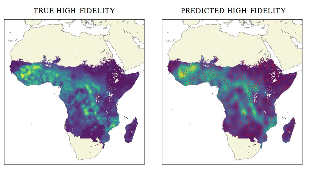
Geostatistics
- Interpolate geospatial fields: rainfall, mineral deposits, temperature, infection spread, etc.
- Closed-form uncertainty \(\to\) principled gap-filling
Protein Stability Prediction
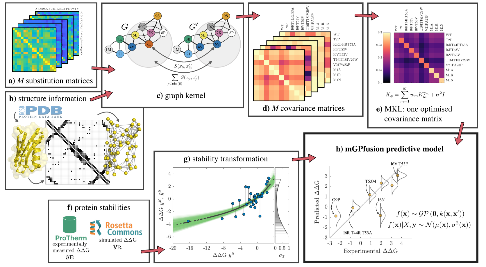
- Measuring protein stability is slow and costly — only a few hundred labeled examples
- GPs thrive in the small-data regime with principled uncertainty
Challenges in modern Gaussian Processes
Challenges in modern Gaussian Processes
Scalability: Gaussian processes have \(\mathcal O(N^3)\) complexity in the number of data points \(N\).
- Solutions: subsets of data, kernel approximations, inducing points, random Fourier features, etc.
Non-Gaussian likelihoods: Exact Gaussian processes assume Gaussian likelihoods, but many real-world datasets have non-Gaussian likelihoods.
- Solutions: approximate inference
Modern Gaussian processes introduce two very different types of approximations:
- Model approximation: for scalability
- Inference approximation: for non-Gaussian likelihoods
Scalable Gaussian Processes
Motivation:
- Gaussian processes have \(\mathcal O(N^3)\) complexity in the number of data points \(N\).
- Above \(N \approx 10,000\) data points, exact Gaussian processes become impractical.
Solution: Find approximations to scale Gaussian processes to large datasets.
Two main approaches:
- Sparse Gaussian processes with inducing points (inspired by the function-space view)
- Kernel approximations using random Fourier features (inspired by the weight-space view)
Inducing points
Idea: Augment the model with a set of \(M \ll N\) inducing points \({\textcolor{input}{\boldsymbol{Z}}}= \{{\textcolor{input}{\boldsymbol{z}}}_1, \ldots, {\textcolor{input}{\boldsymbol{z}}}_M\}\) with corresponding function values \({\textcolor{latent}{\boldsymbol{u}}}= \{\textcolor{latent}{u}_1, \ldots, \textcolor{latent}{u}_M\}\).
Problem: Somehow, solve the inference problem in this augmented model (which is still Gaussian) on a lower computational budget than the original model.
Is this possible? Is it still possible to get exact inference in this augmented model? At what cost?
Yes, the predictive distribution for a new input \({\textcolor{input}{\boldsymbol{x}}}_\star\) is: \[ p(\textcolor{output}{y}_\star \mid {\textcolor{output}{\boldsymbol{y}}}, {\textcolor{input}{\boldsymbol{X}}}, {\textcolor{input}{\boldsymbol{Z}}}) = {\mathcal{N}}\left(\textcolor{output}{y}_\star \mid {\boldsymbol{k}}_{\star{\textcolor{input}{\boldsymbol{Z}}}}^\top{\boldsymbol{Q}}_{{\textcolor{input}{\boldsymbol{Z}}}{\textcolor{input}{\boldsymbol{Z}}}}^{-1}{\boldsymbol{K}}_{{\textcolor{input}{\boldsymbol{Z}}}{\textcolor{input}{\boldsymbol{X}}}}({\boldsymbol{\Lambda}}+ \sigma^2{\boldsymbol{I}})^{-1}{\textcolor{output}{\boldsymbol{y}}},\; k_{\star\star} - {\boldsymbol{k}}_{\star{\textcolor{input}{\boldsymbol{Z}}}}^\top\left({\boldsymbol{K}}_{{\textcolor{input}{\boldsymbol{Z}}}{\textcolor{input}{\boldsymbol{Z}}}}^{-1} - {\boldsymbol{Q}}_{{\textcolor{input}{\boldsymbol{Z}}}{\textcolor{input}{\boldsymbol{Z}}}}^{-1}\right){\boldsymbol{k}}_{\star{\textcolor{input}{\boldsymbol{Z}}}} + \sigma^2\right) \]
where \({\boldsymbol{Q}}_{{\textcolor{input}{\boldsymbol{Z}}}{\textcolor{input}{\boldsymbol{Z}}}} = {\boldsymbol{K}}_{{\textcolor{input}{\boldsymbol{Z}}}{\textcolor{input}{\boldsymbol{Z}}}} + {\boldsymbol{K}}_{{\textcolor{input}{\boldsymbol{Z}}}{\textcolor{input}{\boldsymbol{X}}}}({\boldsymbol{\Lambda}}+ \sigma^2{\boldsymbol{I}})^{-1}{\boldsymbol{K}}_{{\textcolor{input}{\boldsymbol{X}}}{\textcolor{input}{\boldsymbol{Z}}}}\).
Yes, the computational cost is \(O(NM^2)\), instead of \(O(N^3)\).
Gaussian Processes classification
Gaussian processes can be used for classification problems.
Model the latent function \(f({\textcolor{input}{\boldsymbol{x}}})\) as a Gaussian process and apply sigmoid function to get the probability of the class label: \[ p(\textcolor{output}{y}=1 \mid {\textcolor{input}{\boldsymbol{x}}}) = \sigma(f({\textcolor{input}{\boldsymbol{x}}})) \]
Equivalent to assume the Bernoulli likelihood… \[ p(\textcolor{output}{y}\mid \textcolor{latent}{f}) = \text{Bern}(\textcolor{output}{y}\mid \sigma(\textcolor{latent}{f})) \]
… and factorization \[ p({\textcolor{output}{\boldsymbol{y}}}\mid {\textcolor{latent}{\boldsymbol{f}}}) = \prod_{n=1}^N p(\textcolor{output}{y}_n \mid \textcolor{latent}{f}_n) \]
The posterior predictive distribution is not Gaussian anymore and intractable.
Approximate inference for Gaussian Processes classification
As we did for Bayesian logistic regression, we need to use approximate inference methods.
Laplace approximation:
- Find the mode of the posterior distribution using optimization methods.
- Compute the Hessian at the mode.
- Approximate the posterior distribution as a Gaussian with the mode and the Hessian.
Variational inferece