Deep Generative Models
Advanced Statistical Inference
Generative models
Given training data from an unknown distribution \(p_\text{data}({\textcolor{input}{\boldsymbol{x}}})\), we want to learn a model \(p_\text{model}({\textcolor{input}{\boldsymbol{x}}})\) that approximates the true distribution.
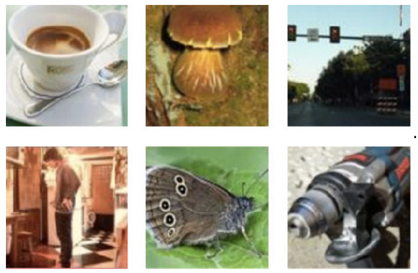
Train from \({\textcolor{input}{\boldsymbol{x}}}\sim p_\text{data}({\textcolor{input}{\boldsymbol{x}}})\).
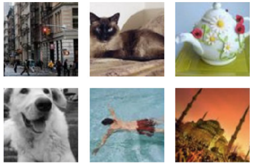
Generate from \({\textcolor{input}{\boldsymbol{x}}}\sim p_\text{model}({\textcolor{input}{\boldsymbol{x}}})\).
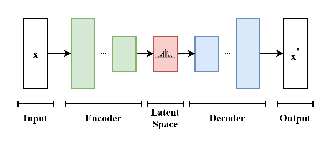
Latent variable models
Our objective is to learn the data distribution \(p({\textcolor{input}{\boldsymbol{x}}})\), but we suppose that each data point \({\textcolor{input}{\boldsymbol{x}}}\) is associated with a latent variable \({\textcolor{latent}{\boldsymbol{z}}}\).
For example, image we want to learn the distribution of images of objects, like the one below:
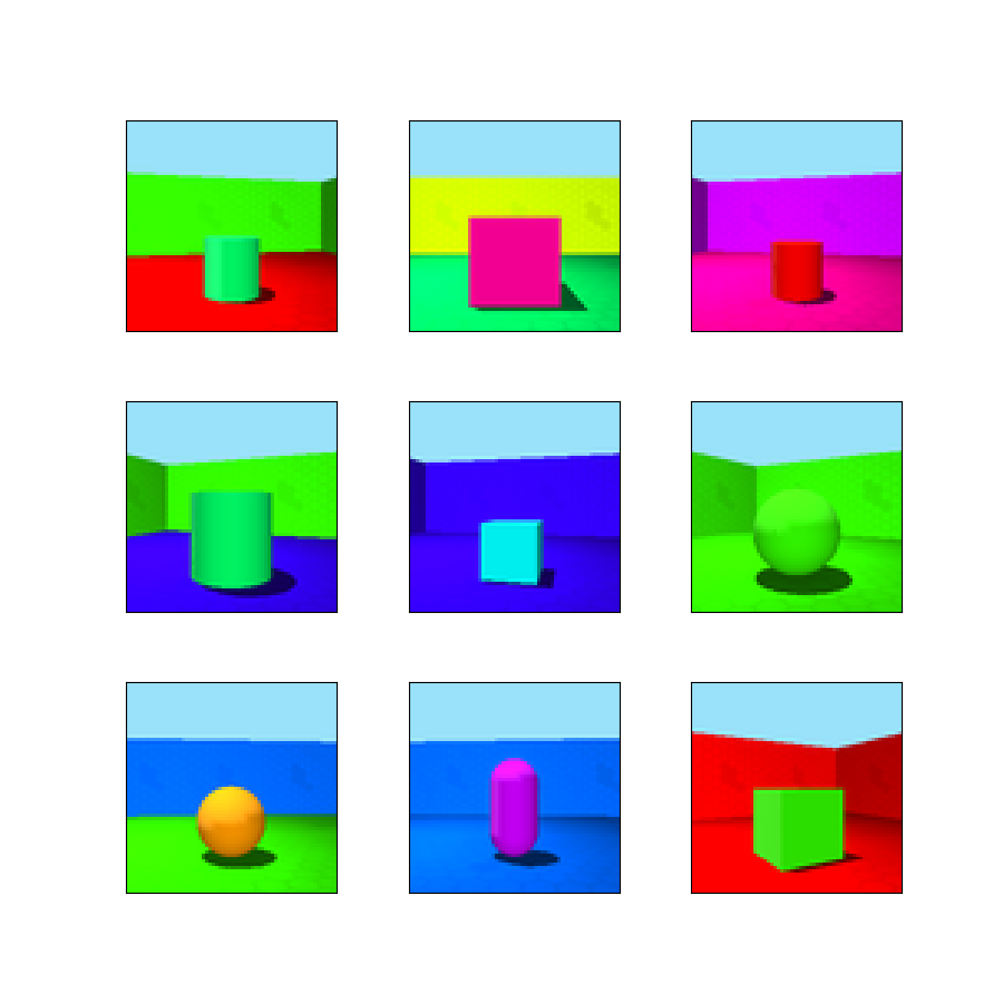
Each image is a huge vector of pixels \({\textcolor{input}{\boldsymbol{x}}}\in \mathbb{R}^{H \times W \times C}\), where \(H\) is the height, \(W\) is the width and \(C\) is the number of channels (in this case, \(64 \times 64 \times 3\)).
Each image can be described by a set of 6 latent variables: floor, wall and object color, shape, orientation and scale.
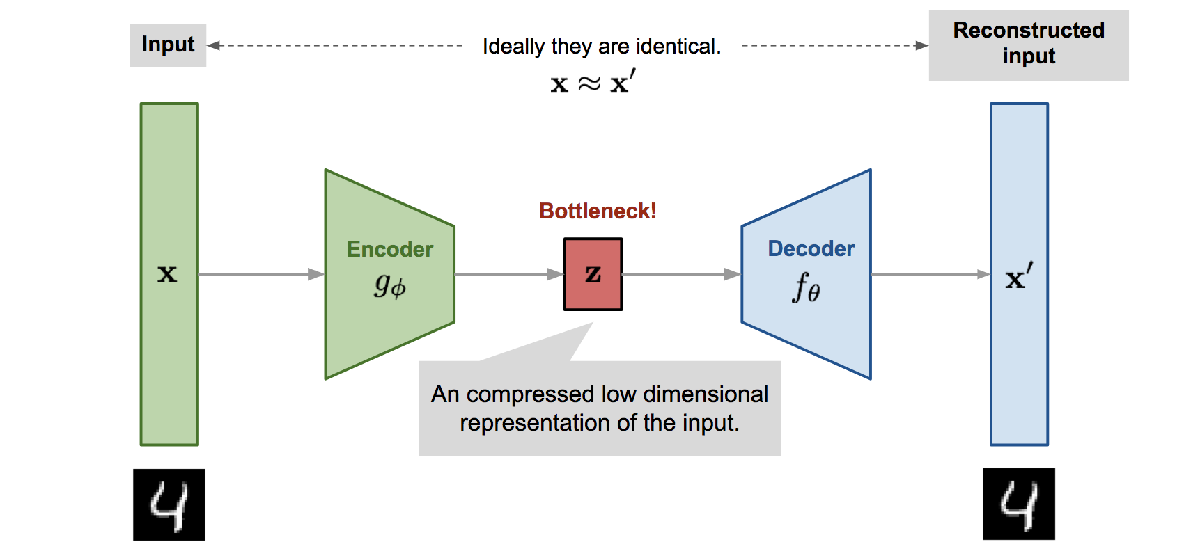
Variational autoencoders (VAEs)
Disclaimer:
Variational autoencoders (VAEs) are often misrepresented as a simple autoencoder with a probabilistic twist.
This is wrong (sort of)! It hides the real nature of the encoder and decoder!
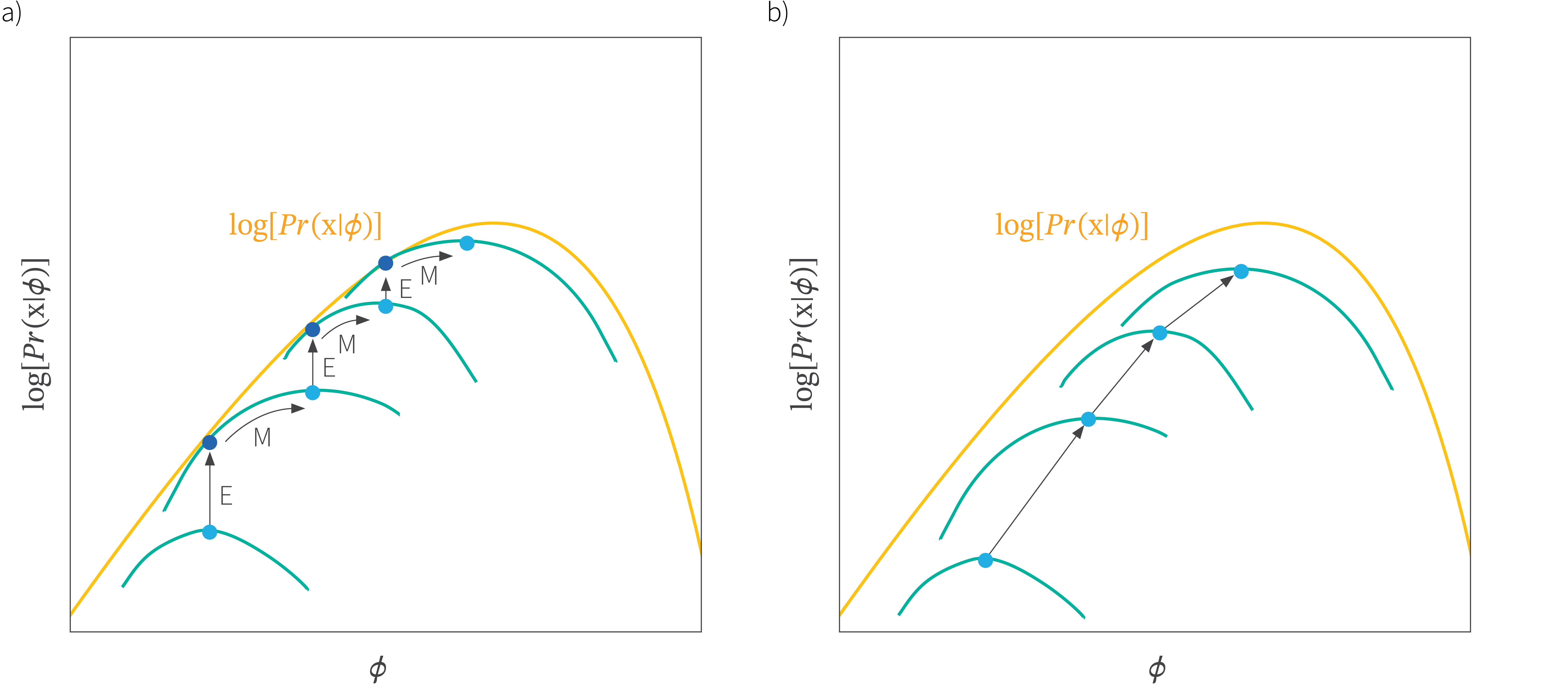
Expectation-Maximization vs Variational Inference
The joint optimization of \({\textcolor{params}{\boldsymbol{\theta}}}\) and \({\textcolor{vparams}{\boldsymbol{\nu}}}\) in VAEs is similar to the Expectation-Maximization (EM) algorithm, but with some key differences:
- In EM, the E-step computes the exact posterior distribution \(p({\textcolor{latent}{\boldsymbol{z}}}\mid {\textcolor{input}{\boldsymbol{x}}}; {\textcolor{params}{\boldsymbol{\theta}}})\), while in VAEs, we approximate it with a variational distribution \(q({\textcolor{latent}{\boldsymbol{z}}}; {\textcolor{vparams}{\boldsymbol{\nu}}})\).
- In EM, the M-step maximizes the exact expected log-likelihood, while in VAEs, we maximize the ELBO, which is a lower bound on the log-likelihood.
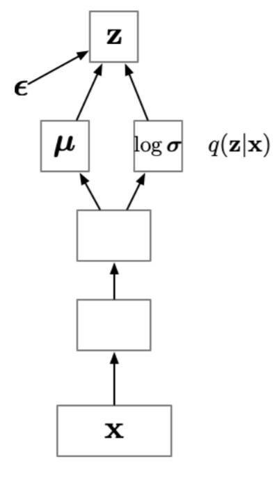
Amortization
Idea: “amortize” the cost of computing the variational parameters \({\textcolor{vparams}{\boldsymbol{\nu}}}\) by learning a function that predicts \(\{ {\boldsymbol{\mu}}, {\boldsymbol{\sigma}}^2 \}\) as a function of the data \({\textcolor{input}{\boldsymbol{x}}}\).
The output of this function is generally \(\textcolor{vparams}{{\boldsymbol{\mu}}}\) and \(\log\textcolor{vparams}{{\boldsymbol{\sigma}}}\) (the \(\log\) is needed to ensure that the variance is positive).
The reparametrization trick is still used to sample from the variational distribution, the only difference is that the variational parameters are not free variables anymore, but are predicted by a neural network \({\boldsymbol{g}}({\boldsymbol{\phi}}, {\textcolor{input}{\boldsymbol{x}}})\).
Sometimes, this is noted as \(q({\textcolor{latent}{\boldsymbol{z}}}\mid {\textcolor{input}{\boldsymbol{x}}})\) to emphasize that the variational distribution depends on the data \({\textcolor{input}{\boldsymbol{x}}}\), even though it’s not actually a conditional distribution.
Putting it all together
Conditional VAE (CVAE)
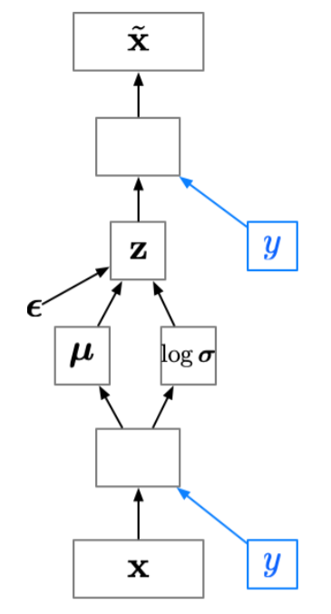
Sometimes we want to generate samples conditioned on some additional information \(p({\textcolor{input}{\boldsymbol{x}}}\mid {\textcolor{output}{\boldsymbol{y}}})\), e.g., we want to generate images of a specific class.
Since the latent code \({\textcolor{latent}{\boldsymbol{z}}}\) no longer has to model the image category, it can focus on modeling the stylistic features.
If we’re lucky, this lets us disentangle style and content. (Note: disentanglement is still a dark art.)
Conditional VAE can be achieve by adding an additional input to the encoder and decoder networks, which is the additional information \({\textcolor{output}{\boldsymbol{y}}}\):
Latent space analysis
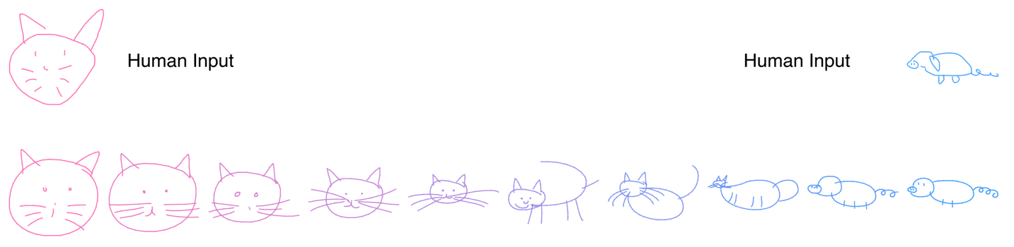
You can often get interesting results by interpolating between two vectors in the latent space:
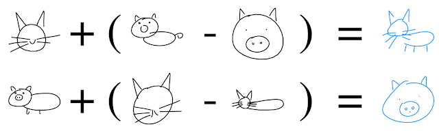
You can also perform “arithmetic” in the latent space, e.g. by adding or subtracting vectors:
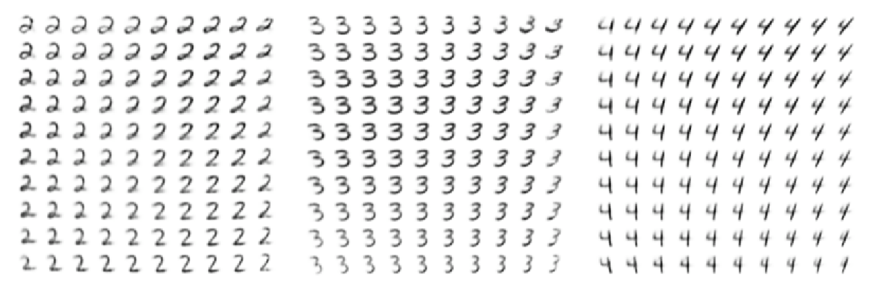
Latent space visualization
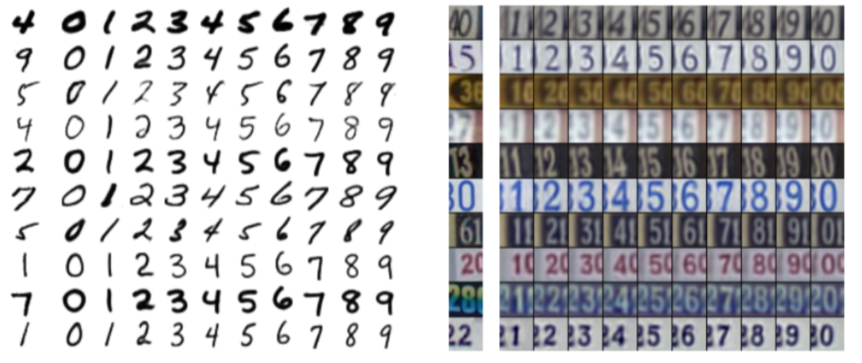
By varying two latent dimensions (i.e. dimensions of \({\textcolor{latent}{\boldsymbol{z}}}\)) while holding \({\textcolor{output}{\boldsymbol{y}}}\) fixed, we can visualize the latent space.
Latent space interpolation
By varying the label \({\textcolor{output}{\boldsymbol{y}}}\) while holding \({\textcolor{latent}{\boldsymbol{z}}}\) fixed, we can solve image analogies.
Problems with VAEs
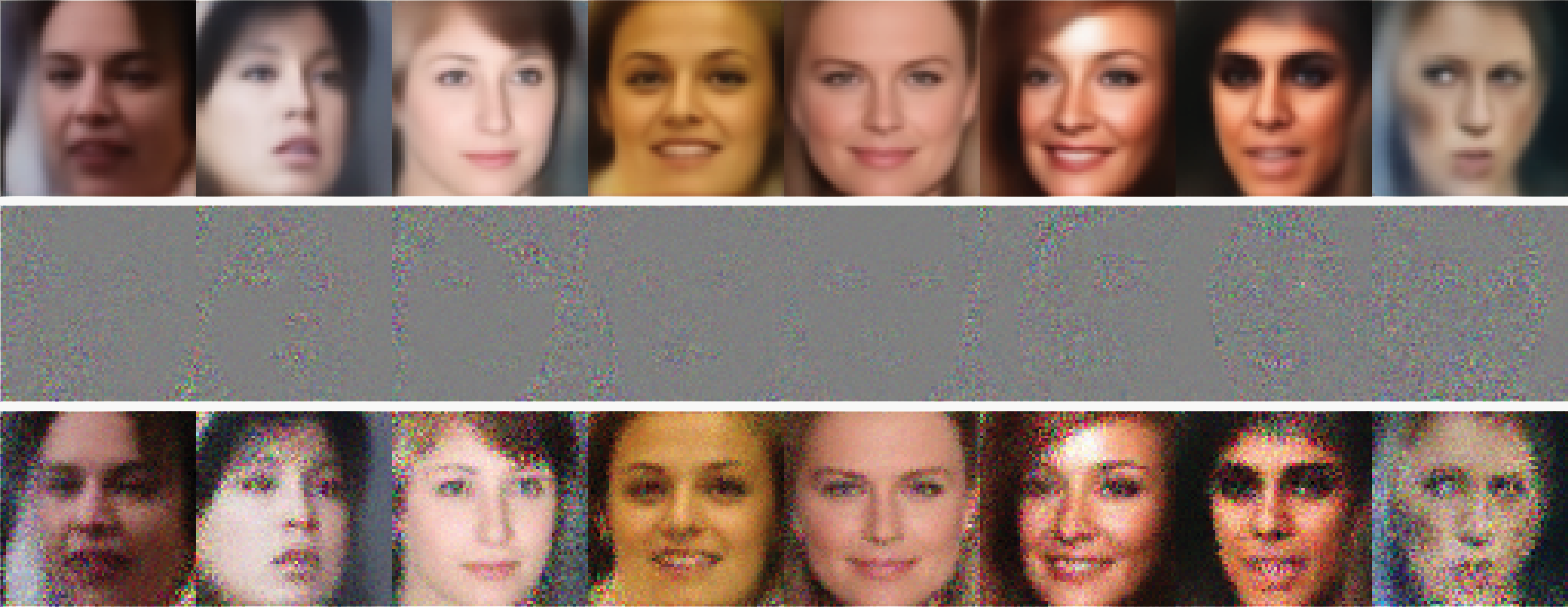
The samples may not be very good:
VAEs suffer from mode collapse, where the amortization network learns to predict the prior. This is due to the strong effect of the KL divergence term in the ELBO.
The spherical prior \(p({\textcolor{latent}{\boldsymbol{z}}})\) is too restrictive, it can lead to a “blurry” output distribution (or very noisy samples, if we sample from the likelihood).