Likelihood-Free Generative Models
Advanced Statistical Inference
Likelihood models
So far we have focused on likelihood-based generative models, where we maximize the likelihood of the data given the model parameters.
Likelihood-based models are powerful, but they have some limitations:
- We run on the assumption that higher likelihood means better generated samples, but this is not always true.
![]()
- We run on the assumption that higher likelihood means better generated samples, but this is not always true.
Likelihood-free learning consider alternative training objectives that do not depend directly on a likelihood
Comparing distributions via samples
\(S_1 = \{ {\textcolor{input}{\boldsymbol{x}}}_1, \ldots, {\textcolor{input}{\boldsymbol{x}}}_N \mid {\textcolor{input}{\boldsymbol{x}}}_i \sim p({\textcolor{input}{\boldsymbol{x}}}) \}\)
\(S_2 = \{ {\textcolor{input}{\boldsymbol{x}}}_1, \ldots, {\textcolor{input}{\boldsymbol{x}}}_N \mid {\textcolor{input}{\boldsymbol{x}}}_i \sim q({\textcolor{input}{\boldsymbol{x}}}) \}\)
Given a finite set of samples from two distributions (\(S_1\) and \(S_2\)), how can we tell if these samples are from the same distribution or not?
Generative models and two-sample tests
Assume \(p_\text{data}({\textcolor{input}{\boldsymbol{x}}})\) is the true data distribution and we have training samples \(S_1\)
Assume we have a model \(p({\textcolor{input}{\boldsymbol{x}}}; {\textcolor{params}{\boldsymbol{\theta}}})\) that permits us to generate samples for \(S_2\)
Idea: formulate the training of the generative model to minimize a two-sample test statistic between \(S_1\) and \(S_2\)
Two-sample tests are hard
In the generative model setup, we know that \(S_1\) and \(S_2\) come from different complex distributions, \(p_\text{data}({\textcolor{input}{\boldsymbol{x}}})\) and \(p({\textcolor{input}{\boldsymbol{x}}}; {\textcolor{params}{\boldsymbol{\theta}}})\). Simple test statistics based on moments (e.g., mean, variance) may not be able to distinguish between the two distributions.
Idea: Learn a statistic to automatically identify in what way the two sets of samples differ
How? Train a classifier (which we will call discriminator)
Discriminator
Build binary classifier \(\textcolor{function}{D}({\textcolor{params}{\boldsymbol{\phi}}}, {\textcolor{input}{\boldsymbol{x}}})\) (e.g., neural network with parameters \({\textcolor{params}{\boldsymbol{\phi}}}\)) that tries to distinguish “real” (\(\textcolor{output}{y}= 1\)) samples from the dataset and “fake” (\(\textcolor{output}{y}= 0\)) samples generated from the model
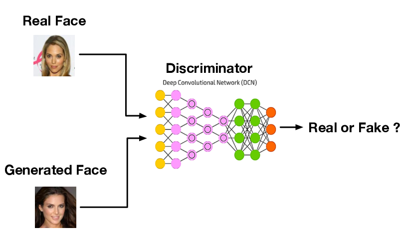
Test statistic: negative loss of the classifier.
- Low loss means real and fake samples are easy to distinguish (distributions are different).
- High loss means real and fake samples are hard to distinguish (distributions are similar).
Goal: Maximize the two-sample test statistic or equivalently minimize the classification loss.
Generator
Still missing: how do we generate the “fake” samples \(S_2\) from the model \(p({\textcolor{input}{\boldsymbol{x}}}; {\textcolor{params}{\boldsymbol{\theta}}})\)?
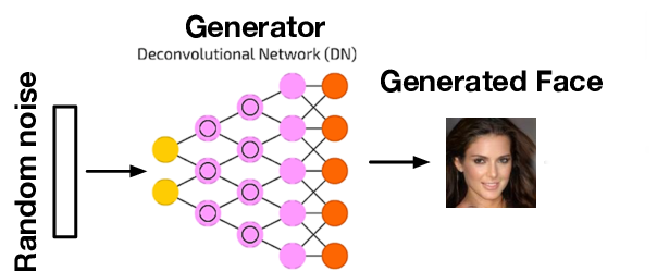
Generator:
Latent variable model with a deterministic mapping from a latent variable \({\textcolor{latent}{\boldsymbol{z}}}\) to the data space \({\textcolor{input}{\boldsymbol{x}}}\):
- Define a function \(\textcolor{function}{G}({\textcolor{params}{\boldsymbol{\theta}}}, {\textcolor{latent}{\boldsymbol{z}}})\) as a neural network with parameters \({\textcolor{params}{\boldsymbol{\theta}}}\)
- Sample \({\textcolor{latent}{\boldsymbol{z}}}\sim p({\textcolor{latent}{\boldsymbol{z}}})\), where \(p({\textcolor{latent}{\boldsymbol{z}}})\) is the prior distribution (e.g., Gaussian)
- Compute \({\textcolor{input}{\boldsymbol{x}}}= \textcolor{function}{G}({\textcolor{params}{\boldsymbol{\theta}}}, {\textcolor{latent}{\boldsymbol{z}}})\),
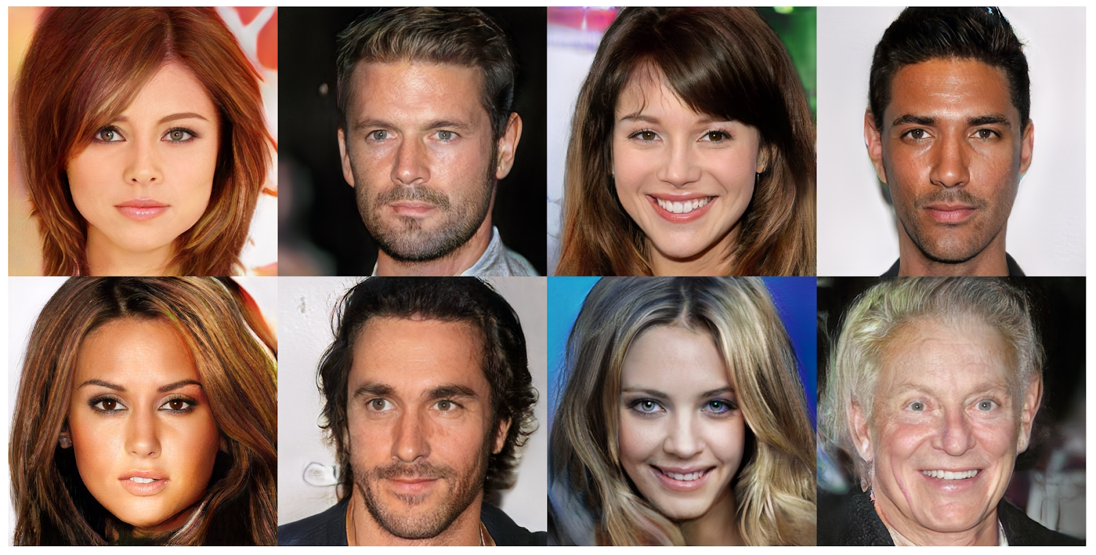
Generative adversarial networks (GANs)
This model configuration and training procedure is known as Generative Adversarial Networks (GANs)
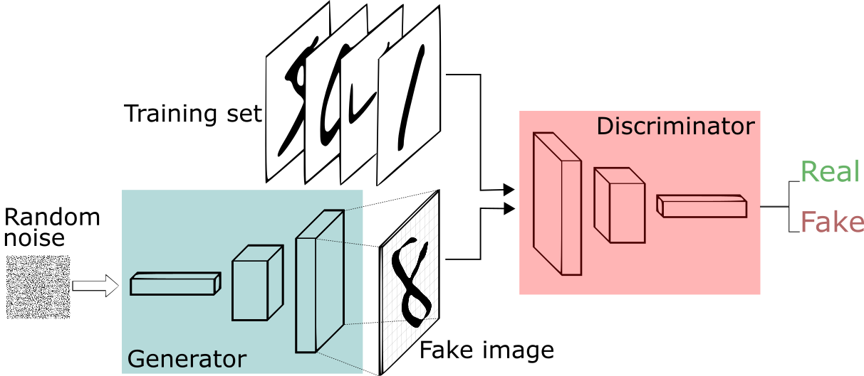
Generative adversarial networks (GANs)
GANs have been successfully applied to several domains and tasks
Training GANs is hard (example)
Imagine \(f(x, y) = xy\) and we want to comput \(\min_x \max_y f(x, y)\). A gradient descent-ascent algorithm would look like this:
\[ \begin{aligned} x &\gets x - \eta \nabla_x f(x, y) = x - \eta y\\ y &\gets y + \eta \nabla_y f(x, y) = y + \eta x \end{aligned} \]
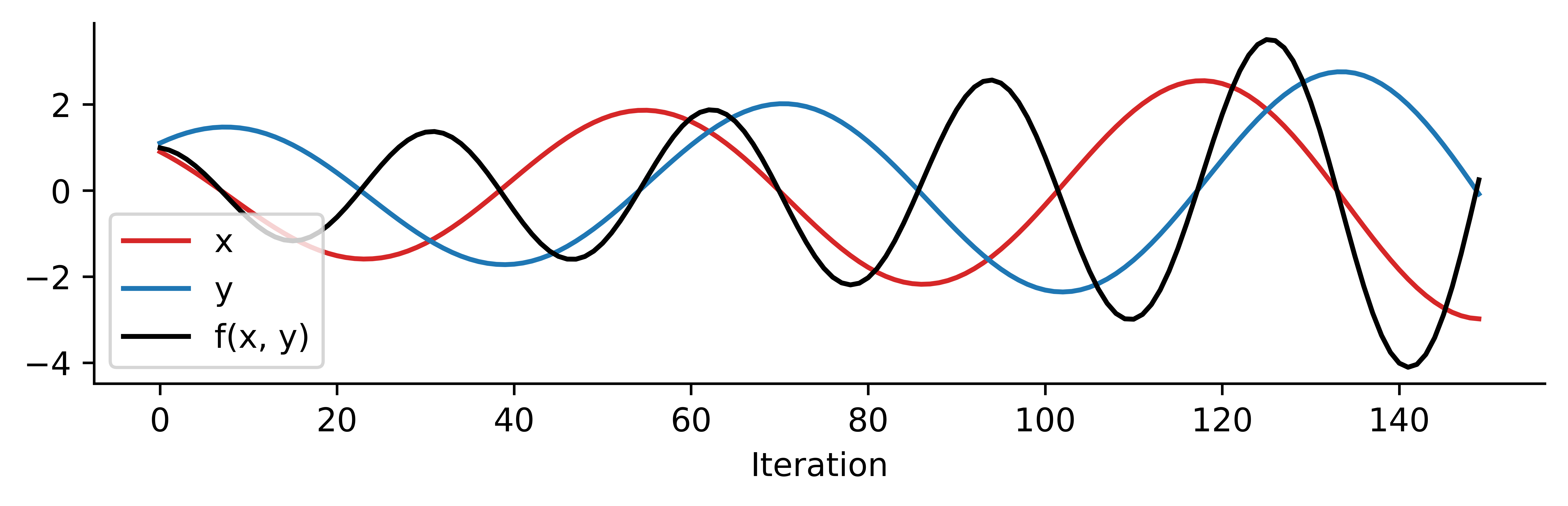
Training GANs is hard
The generator and discriminator loss keep oscillating during GAN training
Difficult to assess if training is converging or not
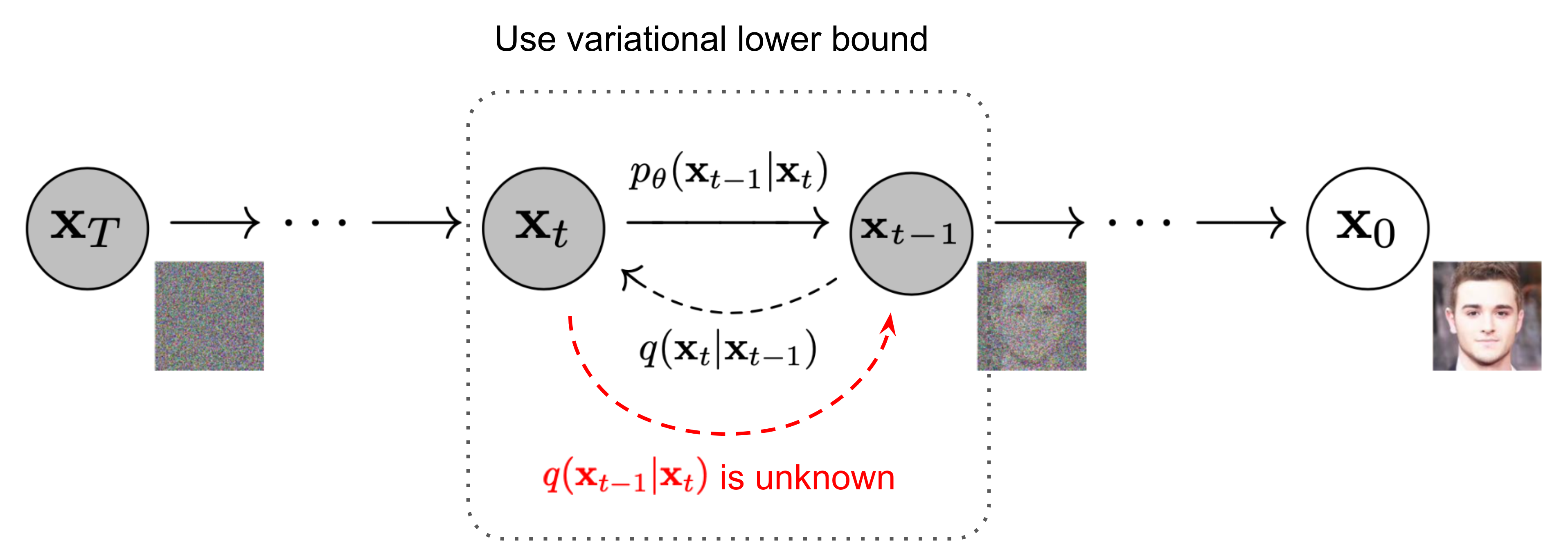
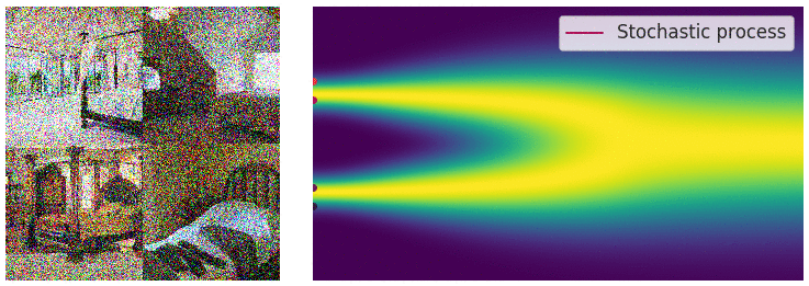
Diffusion models
Currently the state-of-the-art generative models, especially for image/video generation tasks
Diffusion models
Key idea: corrupt the data \({\textcolor{input}{\boldsymbol{x}}}\) into noise by adding Gaussian noise in a series of steps, and then learn to reverse this process to generate new samples.
For example:
\[ q({\textcolor{input}{\boldsymbol{x}}}_t \mid {\textcolor{input}{\boldsymbol{x}}}_{t-1}) = {\mathcal{N}}({\textcolor{input}{\boldsymbol{x}}}_t; \sqrt{1 - \beta_t} {\textcolor{input}{\boldsymbol{x}}}_{t-1}, \beta_t {\boldsymbol{I}}) \]
where \(\beta_t\) is a small positive constant that controls the amount of noise added at each step.
Continuous diffusion process
The diffusion process can be viewed as a continuous-time stochastic process, described by a stochastic differential equation (SDE) of the form:
\[ \dd{\textcolor{input}{\boldsymbol{x}}}_t = {\textcolor{function}{\boldsymbol{f}}}({\textcolor{input}{\boldsymbol{x}}}_t, t) \dd t + g(t) \dd {\boldsymbol{B}}_t \]
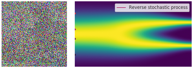
Reverse diffusion process
The reverse diffusion process is also described by an SDE:
\[ \dd{\textcolor{input}{\boldsymbol{x}}}_t = \left({\textcolor{function}{\boldsymbol{f}}}({\textcolor{input}{\boldsymbol{x}}}_t, t) - g(t)^2 \nabla_{{\textcolor{input}{\boldsymbol{x}}}_t} \log p({\textcolor{input}{\boldsymbol{x}}}_t)\right) \dd t + g(t) \dd {\boldsymbol{B}}_t \]
Training diffusion models
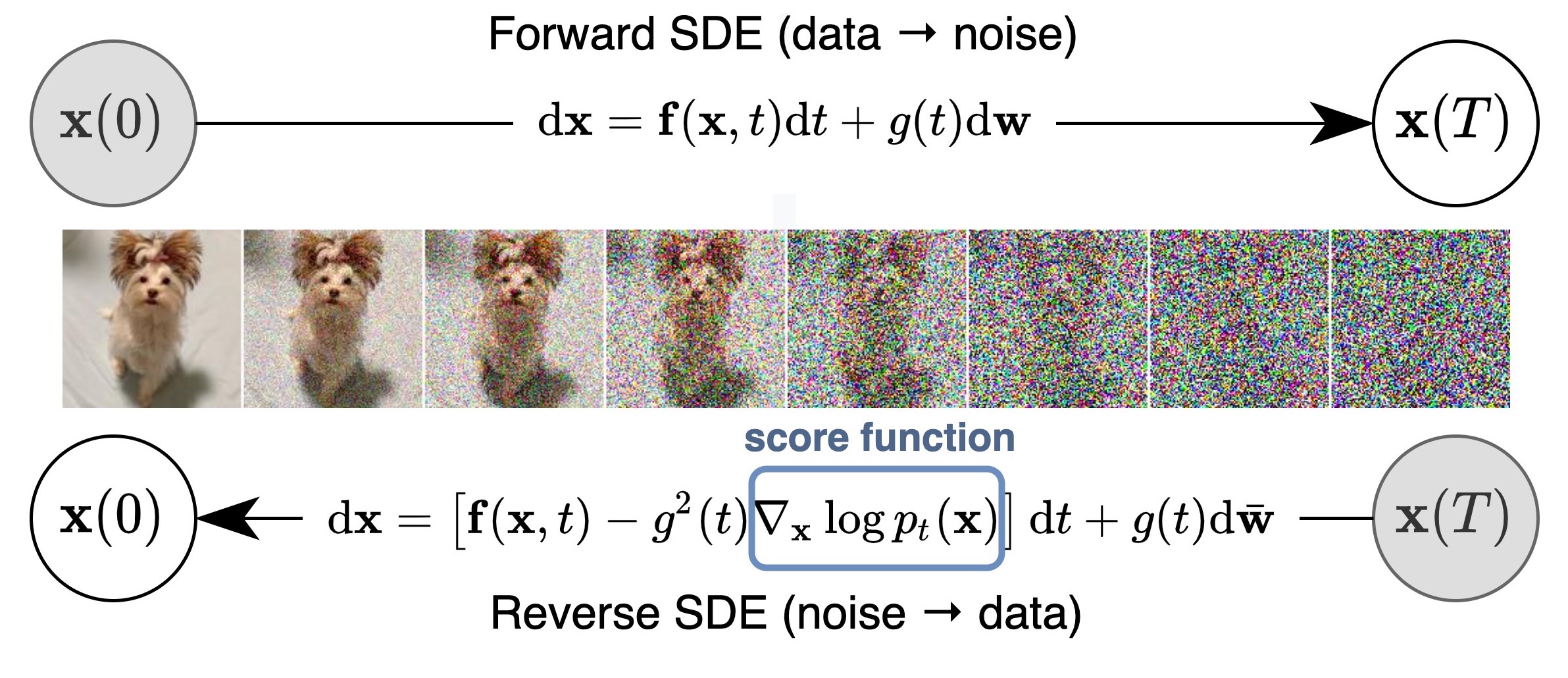
To train the diffusion model, we learn a neural network \({\boldsymbol{s}}({\textcolor{params}{\boldsymbol{\theta}}}, \cdots)\) to approximate the score function \(\nabla_{{\textcolor{input}{\boldsymbol{x}}}_t} \log p({\textcolor{input}{\boldsymbol{x}}}_t)\):
\[ \mathrm{KL}\left( p_0({\textcolor{input}{\boldsymbol{x}}}) \| p({\textcolor{input}{\boldsymbol{x}}}; {\textcolor{params}{\boldsymbol{\theta}}}) \right) \leq \frac{T}{2}\mathbb{E}_{t \in \mathcal{U}(0, T)}\mathbb{E}_{p_t({\textcolor{input}{\boldsymbol{x}}})}[\lambda(t) \| \nabla_{\textcolor{input}{\boldsymbol{x}}}\log p_t({\textcolor{input}{\boldsymbol{x}}}) - {\boldsymbol{s}}({\textcolor{params}{\boldsymbol{\theta}}}, {\textcolor{input}{\boldsymbol{x}}}, t) \|_2^2] + \mathrm{KL}\left( p_T({\textcolor{input}{\boldsymbol{x}}}) \| p_{\text{prior}}({\textcolor{input}{\boldsymbol{x}}}) \right) \]
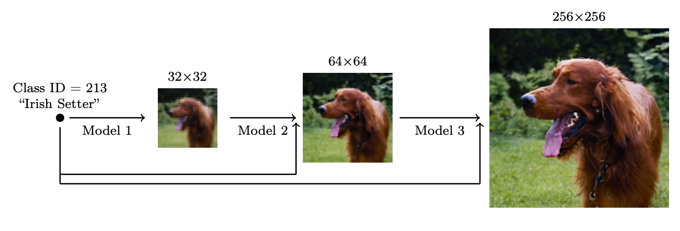
Flexibility of diffusion models: super-resolution
High-resolution samples starting from low-resolution noise:
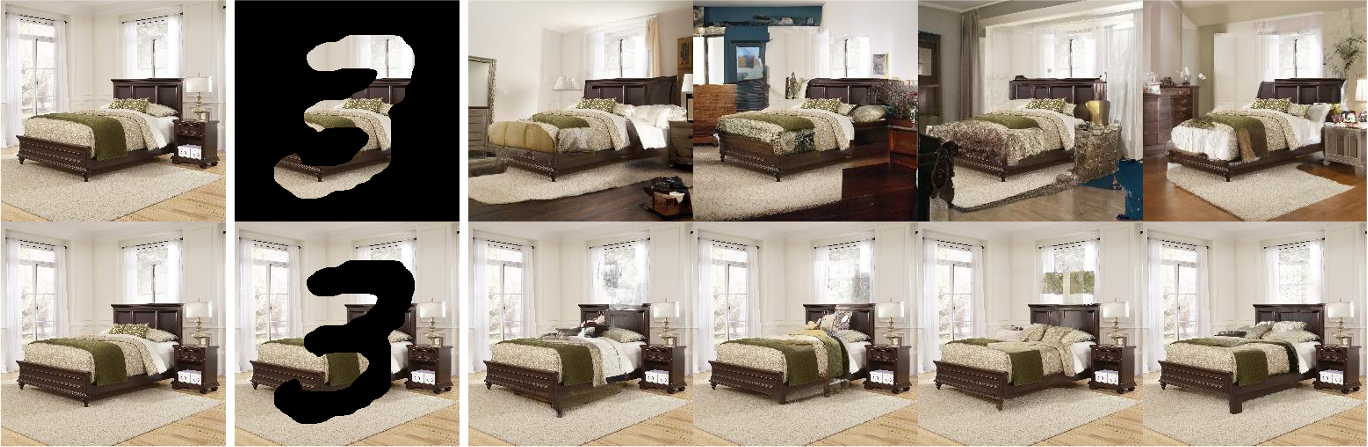
Flexibility of diffusion models: inpainting
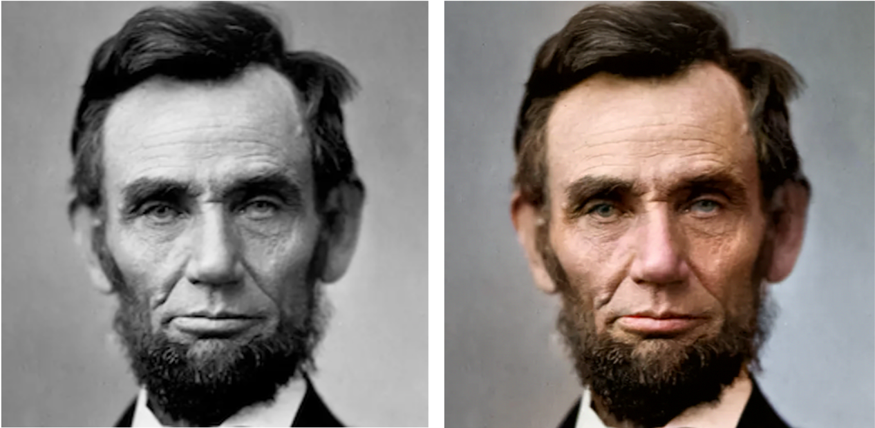
Flexibility of diffusion models: colorization
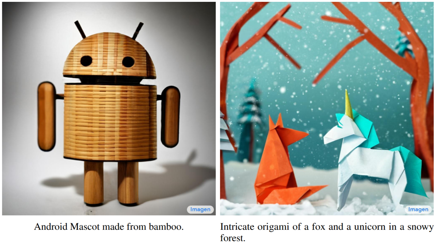
Flexibility of diffusion models: text-to-image

Prompt: Produce a stunning, award-winning close-up of a chameleon blending into a background of vibrant, textured leaves, its eye swivelled to look directly at the camera. The intricate texture of its skin changing colour is the focus (visceral adaptation). Abstract dappled light filters through the leaves. Inspired by wildlife macro photography and camouflage patterns.

Prompt: Cinematic shot using a stabilized drone flying dynamically alongside a pod of immense baleen whales as they breach spectacularly in deep offshore waters. The camera maintains a close, dramatic perspective as these colossal creatures launch themselves skyward from the dark blue ocean, creating enormous splashes and showering cascades of water droplets that catch the sunlight. In the background, misty, fjord-like coastlines with dense coniferous forests provide context. The focus expertly tracks the whales, capturing their surprising agility, immense power, and inherent grace. The color palette features the deep blues and greens of the ocean, the brilliant white spray, the dark grey skin of the whales, and the muted tones of the distant wild coastline, conveying the thrilling magnificence of marine megafauna.